HMMs
Hidden Markov Models
HMMs are probably the most popular directed graphical model out there. They are used in many sequential and temporal domains: speech recognition, handwriting recognition, visual target tracking, machine translation, robot localization, gene prediction, and many more. In HMMs, the random variables are divided into hidden states (phonemes, letters, target location) and observations (audio signal, pen strokes, target image). The goal, as in supervised learning, is to predict the states from observations. For example, guess what this sound wave is saying? Speech recognition is getting better, but there is still a lot to learn. (Try holding a conversation with your phone.)
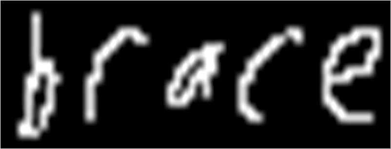
HMMs use the entire sequence of observation to predict the entire sequence of states. While individual observation may be ambiguous:
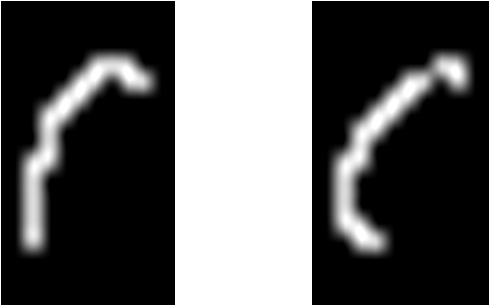
In the context of the entire sequence, the ambiguity is often diminished.
Let's start with the simplest HMM, a 2-state, 2-observation model of the world:
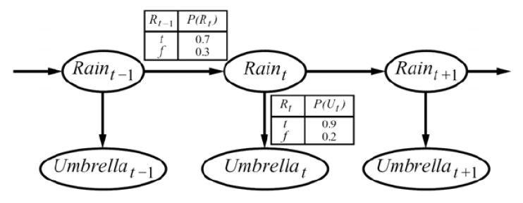
To define this HMM, we need:
- Initial distribution: {$P(R_1)$} - probability of rain on day 1
- Transition distribution: {$P(R_t \mid R_{t-1})$} - probability of rain on day t given rain/no-rain yesterday
- Emission distribution: {$P(U_t \mid R_{t})$} - probability of bringing an umbrella on day t given rain/no-rain
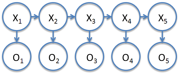
More generally, we will denote the hidden states as {$X_i$} and observations as {$O_i$}. Hidden Markov Models with continuous hidden state and continuous observations are called Kalman Filters. We focus on the discrete states here.
We will use the .. notation to denote a sequence and T to denote the length of the sequence and K the number of values that each state {$X_i$} can take.
- {$X_{i..j}$}: the sequence of variables {$\{X_i,\ldots,X_j\}$}.
- {$x_{i..j}$}: the sequence of assignments {$\{x_i,\ldots,x_j\}$}.
- {$X_{1..T}$}: the entire sequence of states
- {$O_{1..T}$}: the entire sequence of observations
With this notation, the HMM represents the joint probability over states and observations:
{$ \begin{array}{l} P(X_{1..T} = x_{1..T},O_{1..T} = o_{1..T}) = \\ \quad\quad\prod_{i=1}^T P(X_i=x_i \mid X_{i-1} = x_{i-1}) P(O_i=o_i \mid X_i=x_i) \end{array} $}
where {$P(X_1=x_1 \mid X_{0}=x_0) = P(X_1=x_1)$} for convenience of notation.
Conditional Independencies in HMMs
- {$(X_{i-1} \bot X_{i+1} \mid X_{i})$}: the future is independent of the past given the present
- {$(O_{i} \bot X_{i+1} \mid X_{i})$}: the present state fully determines the emission
- {$\neg (O_{i} \bot O_{i+1})$}, but {$(O_{i} \bot O_{i+1} \mid X_i)$} and {$(O_{i} \bot O_{i+1} \mid X_{i+1})$}