HMMInference
Inference in HMMs
Common inference tasks in an HMM are:
- Viterbi decoding (most probable explanation): {$\arg\max_{x_{1..T}} P(X_{1..T}=x_{1..T},O_{1..T}=o_{1..T})$}
- Forward-Backward (computing marginals): {$P(X_i=x_i \mid O_{1..T}=o_{1..T})$}
- Filtering (computing online marginals): {$P(X_i=x_i \mid O_{1..i}=o_{1..i})$}
All of these are computed via a form of dynamic programming.
Forward-Backward
We can use Variable Elimination for each variable {$X_i$}, which would lead to {$O(T^2)$} computations (assuming we picked the right elimination ordering.)
However, we can compute all the marginals in just {$O(T)$} time by dynamic programming. The algorithm computes two values for each position and state in the sequence, {$\alpha_i(x_i) = P(X_i=x_i,o_{1..i})$} and {$\beta_i(x_i) = P(o_{i+1..T} \mid X_i=x_i)$} for {$i=1..T$} and {$x_i = 1..K$}. In words, {$\alpha_i(x_i)$} is the probability of the observed sequence from 1 to i with the i'th state variable equal to {$x_i$}, with the rest of states from 1 to i-1 summed out. On the other hand, {$\beta_i(x_i)$} is the probability of the observed sequence from i+1 to T given that i'th state variable is equal to {$x_i$}. For any state variable {$X_i$}, and state value {$x_i$}, the product of {$\alpha_i(x_i)\beta_i(x_i) = P(X_i=x_i,o_{1..i})P(o_{i+1..T} \mid X_i=x_i)$} is exactly {$P(x_i,o_{1..T})$}. Why? Because
{$ \; \begin{align*} P(x_i,o_{1..T}) & = P(x_i,o_{1..i}) P( o_{i+1..T} \mid x_i,o_{1..i}) \\ & = P(x_i,o_{1..i})P(o_{i+1..T} \mid x_i) \end{align*} \; $}
where the last step is uses the conditional independence assumptions of the HMM. Note that we can compute {$\alpha_i(x_i)$} recursively, because
{$ \; \begin{align*} P(x_i,o_{1..i}) & = \sum_{x_{i-1}} P(x_i,x_{i-1}, o_{1..i}) \\ & = \sum_{x_{i-1}} P(o_i \mid x_i, x_{i-1}, o_{1..i-1}) P(x_i \mid x_{i-1},o_{1..i-1}) P(x_{i-1}, o_{1..i-1}) \\ & = \sum_{x_{i-1}} P(o_i \mid x_i)P(x_i \mid x_{i-1}) P(x_{i-1}, o_{1..i-1}) \end{align*} \; $}
where in the last step we used conditional independence for the first two terms. Similar argument but backwards works for {$\beta_i(x_i)$}.
{$ \; \begin{align*} P(o_{i+1..T} | x_i ) &=\sum_{x_{i+1}}P(o_{i+1..T},x_{i+1}|x_i) =\sum_{x_{i+1}}P(o_{i+1},o_{i+2..T},x_{i+1}|x_i)\\ & =\sum_{x_{i+1}} P(o_{i+1}|o_{i+2..T}, x_{i+1}, x_i) P(o_{i+2..T}| x_{i+1}, x_i) P(x_{i+1} | x_i ) \\ & =\sum_{x_{i+1}} P(o_{i+1}|x_{i+1})P(o_{i+2..T}|x_{i+1}) P(x_{i+1} | x_i)\end{align*} \; $}
Finally, to compute the marginal {$P(x_i \mid o_{1..T})$}, we need to renormalize over all state values {$x_i$} at position i.
Forward-Backward
- Init: {$ \begin{array}{rcl} \alpha_1(x_1) & = & P(o_1 \mid x_1)P(x_1),\;\;\; x_1=1\ldots K\;\; \\ \beta_T(x_T) & = & 1,\;\;\; x_T=1\ldots K \end{array} $}
- (Forward:) For {$i=2\ldots T$}
- {$\alpha_i(x_i) = \sum_{x_{i-1}} P(o_i \mid x_i)P(x_i \mid x_{i-1}) \alpha_{i-1}(x_{i-1}), \;\;\; x_i=1\ldots K$}
- (Backward:) For {$i=T-1\ldots 1$}
- {$\beta_i(x_i) = \sum_{x_{i+1}} P(o_{i+1} \mid x_{i+1}) P(x_{i+1} \mid x_{i}) \beta_{i+1}(x_{i+1}), \;\;\; x_i=1\ldots K$}
- For any i and {$x_i$}, {$P(x_i,o_{1..T}) = \alpha_i(x_i)\beta_i(x_i)$}
The algorithm can be thought of as operating on the lattice of possible values for each hidden variable {$X_i$}. Below is a diagram illustrating an HMM for T steps with K possible hidden state values:
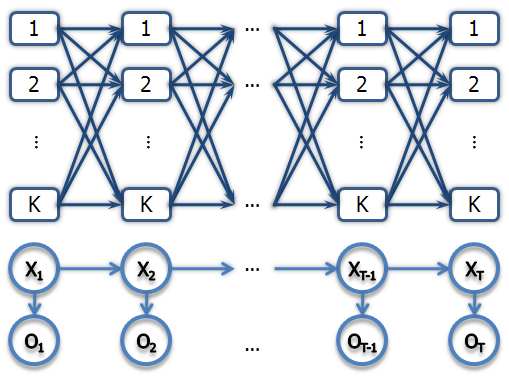
For each rectangular node, the forward pass computes the {$\alpha$} values by combining {$\alpha$} from the previous step with the transition and emission probabilities. The backward pass does the same in reverse.
Viterbi
A similar algorithm can be used to compute {$x_{1..T}^*=\arg\max_{x_{1..T}} P(x_{1..T} \mid o_{1..T})$}. The algorithm computes two values for each position and state in the sequence, {$\delta_i(x_i) = \max_{x_{1..i-1}} P(x_{1..i},o_{1..i})$} and {$\psi_i(x_i)$} (back-pointer) for {$i=1..T$} and {$x_i = 1..K$}. In words, {$\delta_i(x_i)$} is the probability of the observed sequence from 1 to i with the most likely assignment of state variables up to {$i-1$} and the variable {$X_i$} equal to {$x_i$}. {$\psi_i(x_i)$} keeps track of which state for the previous position led to the maximum for state {$x_i$} at the current position.
Viterbi
- Init: {$ \begin{array}{rcl} \delta_1(x_1) & = & P(o_1 \mid x_1)P(x_1),\;\;\; x_1=1\ldots K\;\; \\ \psi_1(x_1) & = & 0,\;\;\; x_1=1\ldots K \end{array} $}
- (Forward:) For {$i=2\ldots T$}
- {$\delta_i(x_i) = \max_{x_{i-1}} P(o_i \mid x_i)P(x_i \mid x_{i-1}) \delta_{i-1}(x_{i-1}), \;\;\; x_i=1\ldots K$}
- {$\psi_i(x_i) = \arg\max_{x_{i-1}} P(o_i \mid x_i)P(x_i \mid x_{i-1}) \delta_{i-1}(x_{i-1}), \;\;\; x_i=1\ldots K$}
- {$P(x^*_{1..T},o_{1..T}) = \max_{x_T}\delta_T(x_T)$}; {$x^*_T = \arg\max_{x_T} \delta_T(x_T)$}.
- (Backtrack:) For {$i=T-1\ldots 1$}
- {$x^*_i = \psi_{i+1}(x^*_{i+1})$}
Parameter Estimation
We will focus on learning HMMs with discrete state space. Suppose we're given labeled sequences of {$(o^i_{1..T_i}, x^i_{1..T_i})$}, {$i=1..n$} to estimate {$P(X_1), P(X_j \mid X_{j-1}), P(O_j \mid X_j)$}. Assuming the observation space is discrete, let's denote the corresponding parameters as: {$\theta_{x}, \theta_{x \mid x'}, \theta_{o \mid x}$}. If the number of hidden states is K and the number of observations is M, then we have {$K+K^2+ KM$} parameters (because of normalization constraints, the number of degrees of freedom is actually {$K-1+ K(K-1)+ K(M-1)$}). The data likelihood is:
{$ \; \begin{align*} \sum_i & \log P(o^i_{1..T_i}, x^i_{1..T_i}) \\ & = \sum_i \log \prod_{j=1}^{T_i} P(X^i_j=x^i_j \mid X^i_{j-1}=x^i_{j-1})P(O^i_j = o^i_j \mid X^i_j = x^i_j) \end{align*} \; $}
Distributing the log inside the product we get:
{$ \; \begin{align*} \sum_i \sum_{j=1}^{T_i} & \log P(X^i_j=x^i_j \mid X^i_{j-1}=x^i_{j-1}) + \\ & \sum_i \sum_{j=1}^{T_i} \log P(O^i_j = o^i_j \mid X^i_j = x^i_j) \end{align*} \; $}
So we can estimate the transition and emission probabilities separately. Let's look at the emission parameters in detail (the others are similar). For each hidden state {$x$}, there are {$M-1$} free parameters, one for each possible observation minus the sum to 1 constraint. Note that we can estimate parameters {$\theta_{o \mid x}$} separately for each state {$x$}, because the objective can be written as a sum over possible hidden states:
{$ \; \begin{align*} \sum_i \sum_{j=1}^{T_i} & \log P(O^i_j = o^i_j \mid X^i_j = x^i_j) \\ & = \sum_{x=1}^K \sum_i \sum_{j=1}^{T_i} \textbf{1}(X^i_j = x)\log P(O^i_j = o^i_j \mid X^i_j = x) \end{align*} \; $}
Essentially, parameter estimation decomposes into estimating each conditional distribution separately. The MLE estimate is simply the relative proportion of each observation in that state:
{$\hat{\theta}_{o \mid x} = \frac{\sum_i\sum_{j=1}^{T_i} \textbf{1}(o^i_{j} = o,x^i_j = x) }{\sum_i\sum_{j=1}^{T_i}\textbf{1}(x^i_{j} = x)}$}
The other parameters are similarly estimated as:
{$ \begin{array}{rcl} \hat{\theta}_{x} & = & \frac{1}{n} \sum_i \textbf{1}(x^i_1 = x) \\ \hat{\theta}_{x \mid x'} & = & \frac{\sum_i\sum_{j=2}^{T_i} \textbf{1}(x^i_{j-1} = x',x^i_j = x) }{\sum_i\sum_{j=2}^{T_i}\textbf{1}(x^i_{j-1} = x')} \end{array} $}
If the observations are continuous, Gaussians are often used to model the distribution {$P(O_j \mid X_j)$}. Let's denote the corresponding parameters as: {$\mu_{x},\sigma_{x}$}.
{$ \; \begin{align*} \hat{\mu}_{x} & = \frac{\sum_i\sum_{j=1}^{T_i} o^i_{j}\textbf{1}(x^i_j = x) }{\sum_i\sum_{j=1}^{T_i}\textbf{1}(x^i_{j} = x)} \\ \hat{\sigma}_{x} & = \frac{\sum_i\sum_{j=1}^{T_i} (\hat{\mu}_x - o^i_{j})^2\textbf{1}(x^i_j = x) }{\sum_i\sum_{j=1}^{T_i}\textbf{1}(x^i_{j} = x)} \end{align*} \; $}
Example: Transition probabilities for POS Tagging in English
As an example, we look at some estimated parameters for the part-of-speech tagging problem. The states are linguistic "tags" like noun (NN), verb (VB), adjective (JJ), determiner (DT), preposition (IN), adverb (RB). At inference time, only words are observed and the goal is to infer the tags.
A subset of the transition probabilities for English part-of-speech tags, computed from a set of 500 sentences, is given below:
Previous\Next     NN        IN        VB        RB        JJ        DT        TO
        NN      0.36      0.24      0.16      0.03      0.01      0.01      0.04
        IN      0.36      0.01      0.05      0.01      0.11      0.35      0.00
        VB      0.15      0.16      0.17      0.11      0.08      0.17      0.07
        RB      0.02      0.14      0.38      0.12      0.14      0.08      0.03
        JJ      0.74      0.08      0.01      0.01      0.10      0.01      0.02
        DT      0.67      0.02      0.03      0.01      0.25      0.01      0.00
        TO      0.11      0.00      0.60      0.00      0.04      0.14      0.00
EM for HMMs
Suppose that we only have unlabeled sequences of observations {$(o^i_{1..T_i})$}, {$i=1..n$} to estimate {$P(X_1), P(X_j \mid X_{j-1}), P(O_j \mid X_j)$} and we would like to learn using EM. We start with a guess at parameters {$\theta^0$} and then iterate inference with weighted MLE. Let
{$q^{t+1}(x^i_j) = P(X^i_j = x^i_j \mid o^i_{1..T_i})$}
using parameters {$\theta^t$}, which can be computed using Forward-Backward. We will also need
{$q^{t+1}(x^i_j,x^i_{j-1}) = P(X^i_j = x^i_j, X^i_{j-1} = x^i_{j-1} \mid o^i_{1..T_i})$}
This is also given by the {$\alpha$} and {$\beta$} of Forward-Backward.
{$P(X_j = x_j, X_{j-1} = x_{j-1} , o_{1..T}) = \alpha_{j-1}(x_{j-1})P(x_j \mid x_{j-1})P(o_j \mid x_{j})\beta_j(x_j)$}
Given the q's, we compute weighted MLE by replacing 1() with q(). (This follows from linearity of expectation).
{$ \; \begin{align*} \hat{\theta}_{x}^{t+1} & = \frac{1}{n} \sum_i q(x^i_1 = x) \\ \hat{\theta}_{x \mid x'}^{t+1} & = \frac{\sum_i\sum_{j=2}^{T_i} q(x^i_{j-1} = x',x^i_j = x) }{\sum_i\sum_{j=2}^{T_i}q(x^i_{j-1} = x')} \\ \hat{\theta}_{o \mid x}^{t+1} & = \frac{\sum_i\sum_{j=1}^{T_i} \textbf{1}(o^i_{j} = o)q(x^i_j = x) }{\sum_i\sum_{j=1}^{T_i}q(x^i_{j} = x)} \end{align*} \; $}
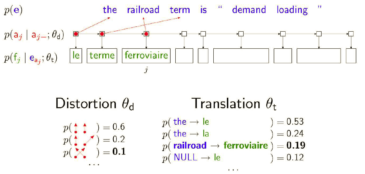
EM is used extensively in learning HMMs for word alignment in machine translation. Given parallel text (pairs of sentences in two languages), the model generates target sentence from source sentence word by word. The alignment variables are hidden and the parameters are learned using EM.
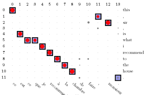
Here is a result of running this model on a corpus of 100K parallel sentences. The marginals {$p(a_i \mid \mathbf{e},\mathbf{f})$} are displayed as circles of size proportional to the posterior probability. The squares indicate correct alignments.
Derivation of EM M-step Updates for HMMs
Let's recall the relevant variables and state what they represent for one particular task --- the optical character recognition (OCR) task from the homework:
| Variable | Meaning | In the OCR context |
|---|---|---|
| {$n$} | # of training examples | # of words |
| {$T_i$} | # of observations comprising example {$i$} | # of letters in the {$i$}th word |
| {$o^i_j$} | value of {$j$}th observation within example {$i$} | {$64$} pixel values |
| {$M$} | # of values an observation can take on | {$2^{64}$} (each pixel can take on value 0 or 1) |
| {$K$} | # of hidden states | the {$26$} letters of the alphabet |
| {$x^i_j$} | value of {$j$}th hidden state for example {$i$} | one of the {$26$} letters of the alphabet |
Suppose we have only unlabeled data {$(o^i_{1..T_i})$}, {$i=1..n$}, that is only pixels (images of letters) but no indication of which letter each image represents. In this case, we aren't able, as in the homework, to simply collect counts of letter labels and the frequency with which each occurs with certain pixels in order to estimate HMM model parameters. We can still try to learn an HMM model of the data to put the images into 26 groups though if we employ the EM algorithm. Recall that the HMM parameters are of three types:
| Parameter type | # of these parameters | In the OCR context |
|---|---|---|
| {$\theta_{x_1} = P(X_1 = x_1)$} | {$K$} | Probability the first letter in a word will be {$x_1$} |
| {$\theta_{x_j \mid x_{j-1}} = P(X_j = x_j \mid X_{j - 1} = x_{j - 1})$} | {$K^2$} | Probability that letter {$x_i$} follows letter {$x_{j - 1}$} |
| {$\theta_{o_j \mid x_j} = P(O_j = o_j \mid X_j = x_j)$} | {$MK$} | Probability of observing the 64 pixels {$o_j$} given someone was writing the letter {$x_j$} |
(Note that in the homework we employed a Naive Bayes assumption so that the observation probabilities decomposed pixel-by-pixel instead of jointly depending on all pixels at once. This significantly reduces the number of observation probabilities that need to be learned.)
To set the value of these parameters using EM, we first make some initial guess at their values, {$\theta^0$}, and run forward-backward to compute initial {$q^0$} values for the E-step (see the HMM EM lecture notes for the exact {$q$} formulas). For all subsequent M-steps ({$t > 0$}), we maximize the following formula, with the hidden state posterior probabilities {$q^t$} held fixed:
{$ \; $ \begin{align*} \theta^{t + 1} = \arg\max_{\theta} & \sum_{i = 1}^n \sum_{x^i_1 = 1}^K q^t(x^i_1) \log (\theta_{x^i_1} \theta_{o^i_1 \mid x^i_1}) + \\ & \sum_{i = 1}^n \sum_{j = 2}^{T_i} \sum_{x^i_j = 1}^K q^t(x^i_j, x^i_{j - 1}) \log (\theta_{x^i_j \mid x^i_{j - 1}} \theta_{o^i_j \mid x^i_j}) \end{align*} $ \; $}
To derive the update formulas for the parameters requires taking derivatives of this expression and setting them to zero.
Update for {$\theta_{x_1}$}
The probabilities associated with the initial distribution, {$\theta_{x_1}$}, only occur in the first term of the expression to be maximized. However, we also have to keep in mind the normalization constraint {$\sum_{x_1 = 1}^K \theta_{x_1} = 1$}. If we add this in using Lagrange multiplier {$\lambda$} then the optimization we need to perform becomes:
{$\min_{\lambda} \max_{\theta_{x_1}} \sum_{i = 1}^n \sum_{x^i_1 = 1}^K q^t(x^i_1) \log (\theta_{x^i_1} \theta_{o^i_1 \mid x^i_1}) - \lambda (\sum_{x_1 = 1}^K \theta_{x_1} - 1)$}
This should all look very familiar to the M-step for {$\pi_k$} at the end of the EM lecture notes. Taking the derivative with respect to {$\theta_{x_1}$} and setting it to zero we obtain:
{$\theta_{x_1} = \frac{1}{\lambda} \sum_{i = 1}^n q^t(x^i_1)$}
To solve for {$\lambda$}, we plug this solution back into the initial formula and eliminate terms that don't include {$\lambda$}:
{$\min_{\lambda} \log (\frac{1}{\lambda}) \sum_{i = 1}^n \sum_{x^i_1 = 1}^K q^t(x^i_1) - \lambda$}
Since {$\sum_{x_1 = 1}^K q^t(x^i_1) = 1$}, this simplifies to: {$\min_{\lambda} n\log (\frac{1}{\lambda}) + \lambda$}. Taking the derivative with respect to {$\lambda$} and setting it equal to zero yields {$\lambda = n$}. Thus, the final update formula for {$\theta_{x_1}$} is:
{$\theta_{x_1} = \frac{1}{n} \sum_{i = 1}^n q^t(x^i_1)$}
This should make intuitive sense; in the OCR setting, it can be interpreted as averaging over the probability mass the posterior {$q^t$} assigns to a particular letter being the first letter in a word.
Update for {$\theta_{x_j \mid x_{j - 1}}$}
The derivation here is very similar to the previous {$\theta_{x_1}$} case. The probabilities associated with the transition distribution, {$\theta_{x_j \mid x_{j - 1}}$}, only occur in the second term of the expression to be maximized though:
{$\max_{\theta_{x_j \mid x_{j - 1}}} \sum_{i = 1}^n \sum_{j = 2}^{T_i} \sum_{x^i_j = 1}^K q^t(x^i_j, x^i_{j - 1}) \log (\theta_{x^i_j \mid x^i_{j - 1}} \theta_{o^i_j \mid x^i_j})$}
As before, we need to augment this objective by considering normalization constraints. In this case, the relevant constraint is: {$\sum_{x_j = 1}^K \theta_{x_j \mid x_{j - 1}} = 1$}. Pushing this into the objective by introducing a Lagrange multiplier {$\nu$} the optimization becomes:
{$ \; $ \begin{align*} \min_{\nu_j} \max_{\theta_{x_j \mid x_{j - 1}}} & \sum_{i = 1}^n \sum_{j = 2}^{T_i} \sum_{x^i_j = 1}^K q^t(x^i_j, x^i_{j - 1}) \log (\theta_{x^i_j \mid x^i_{j - 1}} \theta_{o^i_j \mid x^i_j}) - \\ & \nu \left(\sum_{x_j = 1}^K \theta_{x_j \mid j} - 1\right) \end{align*} $ \; $}
Taking the derivative with respect to one parameter, say {$\theta_{x_j \mid x_{j - 1}} = \theta_{a \mid b}$} where {$a,b \in 1..K$} and setting it equal to zero we obtain:
{$\theta_{a \mid b} = \frac{1}{\nu_b} \sum_{i = 1}^n \sum_{j = 2}^{T_i} q(x^i_j = a, x^i_{j - 1} = b)$}
To solve for {$\nu_b$}, we plug this solution back into the initial formula and eliminate terms that don't include {$\nu_b$}:
{$\min_{\nu_b} \log (\frac{1}{\nu_b}) \sum_{i = 1}^n \sum_{j = 2}^{T_i} \sum_{x^i_j = 1}^K q^t(x^i_j, x^i_{j - 1} = b) - \nu_b \left(\frac{1}{\nu_b} \sum_{x_j = 1}^K q(x_j = a, x_{j - 1} = b) - 1\right)$}
Since {$\sum_{x^i_j = 1}^K q^t(x^i_j, x^i_{j - 1} = b) = q^t(x^i_{j - 1} = b)$}, the first term simplifies to {$-\log(\nu_b) \sum_{i = 1}^n \sum_{j = 2}^{T_i} q^t(x^i_{j - 1} = b)$}. In the first part of the second term, the {$\nu_b$} cancel, so we can consider this term constant and drop it from our {$\min_{\nu_b}$} optimization. The resulting formula is:
{$\min_{\nu_b} -\log(\nu_b) \sum_{i = 1}^n \sum_{j = 2}^{T_i} q^t(x^i_{j - 1} = b) + \nu_b$}
Taking the derivative with respect to {$\nu$} and setting it equal to zero yields {$\nu = \sum_{i = 1}^n \sum_{j = 2}^{T_i} q^t(x^i_{j - 1} = b)$}. Thus, the final update formula for {$\theta_{a \mid b}$} is:
{$\theta_{a \mid b} = \frac{\sum_{i = 1}^n \sum_{j = 2}^{T_i} q(x^i_j = a, x^i_{j - 1} = b)}{\sum_{i = 1}^n \sum_{j = 2}^{T_i} q^t(x^i_{j - 1} = b)}$}