Overfitting
Overfitting and Regularization
In general, overfitting happens when a model learns to describe noise in addition to the real dependencies between input and output. In terms of bias/variance decomposition, a complex model that can achieve very small error on any dataset (it has low bias for any problem) may have large error on new examples (test set) because its variance (dependence on the particular dataset observed) is too high. The applet for polynomial regression illustrates this well.
One way to quantify of the strength of the algorithm dependence on the dataset is to imagine changing the label of a single example in classification or shifting the real-valued outcome of a single example in regression and seeing how much that would affect the learned prediction model. (This measure of sensitivity of the learning algorithm to a change in single example is called stability).
So far we have seen several ways to control model complexity:
- Choice of degree of polynomial in regression to prefer less wiggly models
- Bayesian priors on parameters as a way to prefer smoother models
- Limit on depth of decision trees to prefer simpler models
We will see several more examples of complexity control, also called regularization, soon. Typically, the trade-off is posed as follows:
{$\arg\min_{h\in\mathcal{H}} \textbf{training loss}(h) + C*\textbf{complexity}(h)$}
or
{$\arg\min_{h\in\mathcal{H}} \textbf{training loss}(h) \;\;\; \textbf{such that} \;\;\;\;\textbf{complexity}(h) \leq C$}
where is C is the strength of complexity penalty.
Training Loss vs Complexity trade-off (aka bias/variance)
A common pattern of overfitting is illustrated in this idealized figure:
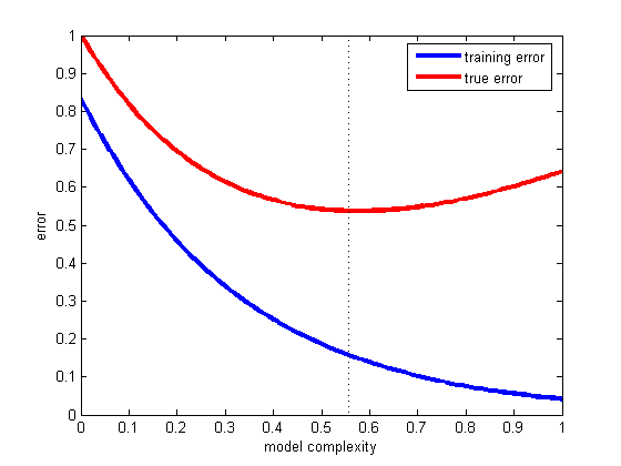
Error vs Complexity trade-off
We focus on classification below, but this entire discussion applies equally well to regression. Recall that training error of a classifier {$h(\mathbf{x})$} on the dataset D of n samples is simple to compute:
{$ \textbf{training error}: \;\; \frac{1}{n} \sum_i \mathbf{1}(h(\mathbf{x}_i)\ne y_i)$}
while the true error of {$h(\mathbf{x})$} depends on the unknown {$P(\mathbf{x},y)$}:
{$ \textbf{true error}: \;\; \mathbf{E}_{(\mathbf{x},y)\sim P}[ \mathbf{1}(h(\mathbf{x})\ne y)]$}
We use a test set, {$D_{test} = \{ \mathbf{x}_i, y_i\}_{n+1}^{n+n_{test}}$} which is not used to select the classifier, as an unbiased estimate of the true error:
{$ \textbf{test set error}: \;\; \frac{1}{n_{test}} \sum_{i=n+1}^{n+n_{test}} \mathbf{1}(h(\mathbf{x}_i)\ne y_i)$}
In the figure above, there is a lowest point in the true error curve where underfitting ends and overfitting begins. This point corresponds to the optimal trade-off between minimizing training error and model complexity.
For a fixed complexity penalty, the learning curve usually looks like this:
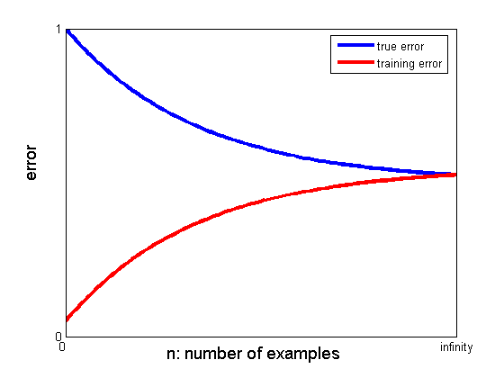
Learning curve
As we increase model complexity, the point where the two curves meet at infinity shifts down, but the gap remains. The key is to choose the right complexity.
Adjusting complexity penalty using cross-validation
How do we set the right amount of complexity control? There are some theoretical guidelines that can help you find ball-park range of complexity, but in practice, the best way to control complexity is by setting aside some of the training data for a validation set, for example a tenth of your data. This validation set is used only to set the complexity penalty (a single parameter, like max depth of a tree, strength of prior in regression) by learning several classifiers on the training set (minus validation), for a set of values of complexity penalty. Each classifier is then tested on the validation set and the classifier with lowest error is selected. As long as the learning algorithm that fits the model (for a given complexity) does not use the validation set, validation set error is an unbiased estimate of the true error.
LOOCV: Leave-one-out cross-validation
When the dataset is very small, leaving one tenth out depletes our data too much, but making the validation set too small makes the estimate of the true error unstable (noisy). One solution is to do a kind of round-robin validation: for each complexity setting, learn a classifier on all the training data minus one example and evaluate its error the remaining example. Leave-one-out error is defined as:
{$\textbf{LOOCV error}: \frac{1}{n} \sum_i \mathbf{1}(h(\mathbf{x}_i; D_{-i})\ne y_i)$}
where {$D_{-i}$} is the dataset minus ith example and {$h(\mathbf{x}_i; D_{-i})$} is the classifier learned on {$D_{-i}$}. LOOCV error is an unbiased estimate of the error of our learning algorithm (for a given complexity setting) when given n-1 examples.
K-Fold cross-validation
When the dataset is large, learning n times number of complexity settings classifiers may be prohibitive. For some models, there are tricks that can make it fast, but for most cases, K-fold cross-validation (with K typically 10) is a practical solution. The idea is simply to split the data into K subsets or folds {$ {D_1} , \ldots, D_K$} and leave out each fold in turn for validation. The K-fold validation error is:
{$\textbf{K-fold validation error}: \frac{1}{n} \sum_{k=1}^K \sum_{i\in D_k} \mathbf{1}(h(\mathbf{x}_i; D-D_k)\ne y_i)$}
where {$D-D_k$} is the dataset minus kth fold and {$h(\mathbf{x}_i; D-D_k)$} is the classifier learned on {$D-D_k$}. Again, this error is an unbiased estimate of the error of our learning algorithm (for a given complexity setting) when given {$n\frac{K-1}{K}$} examples.
Using selected complexity
Both LOOCV and K-fold cross-validation give us a way to find a good setting for regularization. A common practice is to learn a new classifier with that setting on all the data. This is not perfectly justified because the complexity penalty estimate is (slightly) pessimistic: it is estimated for datasets with less data. However, this works out well enough in practice. Another option is to combine the learned classifiers from each fold by averaging (in regression) or voting (in classification) their predictions.
Video
An informative video describing K-fold cross-validation and its use in regularization (model selection) can be found here