NaiveBayes
Naive Bayes Model
The Naive Bayes classifier is an example of the generative approach: we will model {$P(\mathbf{x},y)$}. Consider the toy transportation data below:
| x: Inputs/Features/Attributes | y: Class | ||
|---|---|---|---|
| Distance(miles) | Raining | Flat Tire | Mode |
| 1 mile | no | no | bike |
| 2 miles | yes | no | walk |
| 1 mile | no | yes | bus |
| 1 mile | yes | no | walk |
| 2 miles | yes | no | bus |
| 1 mile | no | no | car |
| 1 mile | yes | yes | bike |
| 10 miles | yes | no | bike |
| 10 miles | no | no | car |
| 4 miles | no | no | bike |
We will decompose {$P(\mathbf{x},y)$} into class prior and class model:
{$P(\mathbf{x},y) = \underbrace{P(y)}_{\rm class prior} \underbrace{P(\mathbf{x}\mid y)}_{\rm class model}$}
and estimate them separately as {$\hat{P}(y)$} and {$\hat{P}(\mathbf{x} \mid y)$}. (Class prior should not be confused with parameter prior. They are very similar concepts, but not the same things.)
We will then use our estimates to output a classifier using Bayes rule:
{$ \begin{align*} h(\mathbf{x}) & = \arg\max_y \;\;\hat{P}(y\mid \mathbf{x}) \\ & = \arg\max_y \;\;\;\; \frac{\hat{P}(y)\hat{P}(\mathbf{x} \mid y)}{\sum_{y'}\hat{P}(y')\hat{P}(\mathbf{x} \mid y')} \\ & = \arg\max_y \;\;\;\; \hat{P}(y)\hat{P}(\mathbf{x} \mid y) \end{align*} $}
To estimate our model using MLE, we can separately estimate the two parts of the model:
{$ \begin{align*} \log P(D) & = \sum_i \log P(\mathbf{x}_i,y_i) \\ & = \sum_i \log P(y_i) + \log P(\mathbf{x}_i \mid y_i) \\ & = \log P(D_Y) + \log P(D_X | D_Y) \end{align*} $}
Estimating {$P(y)$}
How do we estimate {$P(y)$}? This is very much like the biased coin, except instead of two outcomes, we have 4 (walk, bike, bus, car). We need 4 parameters to represent this multinomial distribution (3 really, since they must sum to 1): {$(\theta_{\rm walk},\theta_{\rm bike},\theta_{\rm bus},\theta_{\rm car})$}. The MLE estimate (deriving it is a good exercise) is {$\hat{\theta}_y = \frac{1}{n}\sum_i \textbf{1}(y=y_i)$}.
| y | parameter {$\theta_{y}$} | MLE {$\hat{\theta}_{y}$} |
|---|---|---|
| walk | {$\theta_{\rm walk}$} | 0.2 |
| bike | {$\theta_{\rm bike}$} | 0.4 |
| bus | {$\theta_{\rm bus}$} | 0.2 |
| car | {$\theta_{\rm car}$} | 0.2 |
Estimating {$P(\textbf{x}\mid y)$}
Estimating class models is much more difficult, since the joint distribution of m dimensions of {$\textbf{x}$} can be very complex. Suppose that all the features are binary, like Raining or Flat Tire above. If we have m features, there are {$K*2^m$} possible values of {$(\textbf{x},y)$} and we cannot store or estimate such a distribution explicitly, like we did for {$P(y)$}. The key (naive) assumption of the model is conditional independence of the features given the class. Recall that {$X_k$} is conditionally independent of {$X_j$} given Y if:
{$P(X_j=x_j \mid X_k=x_k, Y=y)= P(X_j=x_j \mid Y=y), \; \forall x_j,x_k,y$}
or equivalently,
{$ \begin{align*} P(X_j=x_j,X_k=x_k\mid Y=y) & = \\ & P(X_j=x_j\mid Y=y)P(X_k=x_k\mid Y=y),\forall x_j,x_k,y \end{align*} $}
More generally, the Naive Bayes assumption is that:
{$\hat{P}(\mathbf{X}\mid Y) = \prod_j \hat{P}(X_j\mid Y)$}
Hence the Naive Bayes classifier is simply:
{$\arg\max_y \hat{P}(Y=y \mid \mathbf{X}) = \arg\max_y \hat{P}(Y=y)\prod_j \hat{P}(X_j\mid Y=y)$}
If the feature {$X_j$} is discrete like Raining, then we need to estimate K distributions for it, one for each class, {$P(X_j | Y = k)$}. We have 4 parameters, ({$\theta_{{\rm R}\mid\rm walk}, \theta_{{\rm R}\mid\rm bike}, \theta_{{\rm R}\mid\rm bus}, \theta_{{\rm R}\mid\rm car}$}), denoting probability of Raining=yes given transportation taken. The MLE estimate (deriving it is also a good exercise) is {$\hat{\theta}_{{\rm R}\mid y} = \frac{\sum_i \textbf{1}(R=yes, y=y_i)}{\sum_i \textbf{1}(y=y_i)}$}. For example, {$P({\rm R}\mid Y)$} is
| y | parameter {$\theta_{{\rm R}\mid y}$} | MLE {$\hat{\theta}_{R \mid y}$} |
|---|---|---|
| walk | {$\theta_{{\rm R}\mid\rm walk}$} | 1 |
| bike | {$\theta_{{\rm R}\mid\rm bike}$} | 0.5 |
| bus | {$\theta_{{\rm R}\mid\rm bus}$} | 0.5 |
| car | {$\theta_{{\rm R}\mid\rm car}$} | 0 |
For a continuous variable like Distance, there are many possible choices of models, with Gaussian being the simplest. We need to estimate K distributions for each feature, one for each class, {$P(X_j | Y = k)$}. For example, {$P({\rm D}\mid Y)$} is
| y | parameters {$\mu_{{\rm D}\mid y}$} and {$\sigma_{{\rm D}\mid y}$} | MLE {$\hat{\mu}_{{\rm D}\mid y}$} | MLE {$\hat{\sigma}_{{\rm D}\mid y}$} |
|---|---|---|---|
| walk | {$\mu_{{\rm D}\mid\rm walk}$},{$\sigma_{{\rm D}\mid\rm walk}$} | 1.5 | 0.5 |
| bike | {$\mu_{{\rm D}\mid\rm bike}$}, {$\sigma_{{\rm D}\mid\rm bike}$} | 4 | 3.7 |
| bus | {$\mu_{{\rm D}\mid\rm bus}$}, {$\sigma_{{\rm D}\mid\rm bus}$} | 1.5 | 0.5 |
| car | {$\mu_{{\rm D}\mid\rm car}$}, {$\sigma_{{\rm D}\mid\rm car}$} | 5.5 | 4.5 |
Note that for words, instead of using a binary variable (word present or absent), we could also use the number of occurrences of the word in the document, for example by assuming a binomial distribution for each word.
MLE vs. MAP
Note the danger of using MLE estimates. For example, consider the estimate of conditional distribution of Raining=yes: {$\hat{P}({\rm Raining = yes} \mid y={\rm car}) = 0$}. So if we know it's raining, no matter the distance, the probability of taking the car is 0, which is not a good estimate. This is a general problem due to scarcity of data: we never saw an example with car and raining. Using MAP estimation with Beta priors (with {$\alpha,\beta>1$}), estimates will never be zero, since additional "counts" are added.
Examples
2-dimensional, 2-class example
Suppose our data is from two classes (plus and circle) in two dimensions ({$x_1$} and {$x_2$}) and looks like this:
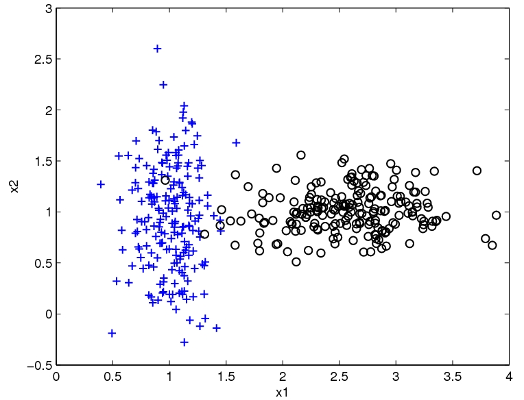
2D binary classification data
The Naive Bayes classifier will estimate a Gaussian for each class and each dimension. We can visualize the estimated distribution by drawing a contour of the density. The decision boundary, where the probability of each class given the input is equal, is shown in red.
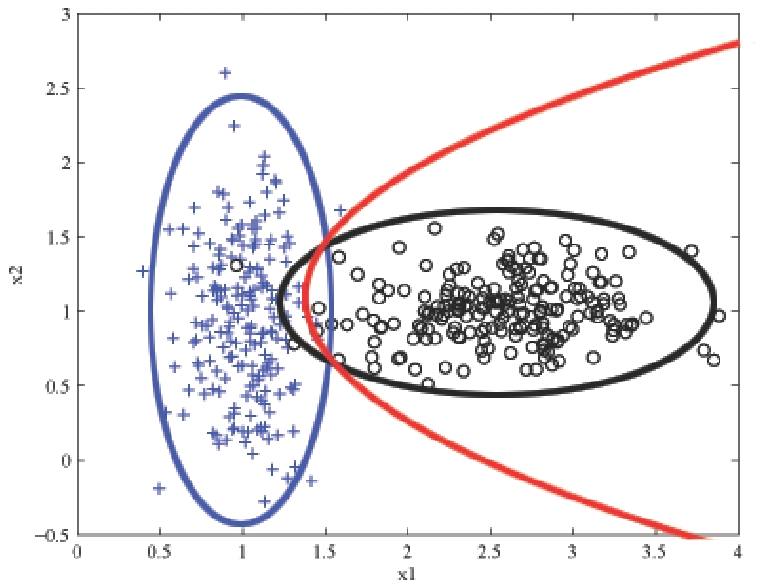
2D binary classification with Naive Bayes. A density contour is drawn for the Gaussian model of each class and the decision boundary is shown in red
Text classification: bag-of-words representation
In classifying text documents, like news articles or emails or web pages, the input is a very complex, structured object. Fortunately, for simple tasks like deciding about spam vs. not spam, politics vs sports, etc., a very simple representation of the input suffices. The standard way to represent a document is to completely disregard the order of the words in it and just consider their counts. So the email below might be represented as:

bag-of-words model for text classification: degree=1, diploma=1, customized=1, deserve=1, fast=1, promptly=1...
The Naive Bayes classifier then learns {$\hat{P}(spam)$}, and {$\hat{P}(word\mid spam)$} and {$\hat{P}(word \mid ham)$} for each word in our dictionary by using MLE/MAP as above. It then predicts prediction 'spam' if:
{$\hat{P}(spam)\prod_{{\rm word} \in {\rm email}} \hat{P}(word\mid spam) > \hat{P}(ham)\prod_{{\rm word} \in {\rm email}} \hat{P}(word\mid ham)$}