MatricesAndTensors
Linear Algebra Review
Vector Basics
For {$m$}-dimensional vectors {$\mathbf{v}$} and {$\mathbf{u}$} that form angle {$\theta$} with each other:
| Property Name | Denotation | Formula |
| Length of {$\mathbf{v}$} | {$|\mathbf{v}|$} or {$||\mathbf{v}||_2$} | {$\sqrt{\sum_{i = 1}^{m} v^2_i}$} |
| Inner (dot) product of {$\mathbf{v}$} and {$\mathbf{u}$} | {$\mathbf{v} \cdot \mathbf{u}$} or {$\mathbf{v}^T \mathbf{u}$} or {$<\mathbf{v}, \mathbf{u}>$} | {$\sum_{i = 1}^m v_i u_i$} or {$|v||u|\cos(\theta)$} |
| Projection of {$\mathbf{v}$} onto {$\mathbf{u}$} | {$\textrm{proj}_{\mathbf{u}}(\mathbf{v})$} | {$<\mathbf{v},\mathbf{u}> \frac{\mathbf{u}}{<\mathbf{u},\mathbf{u}>}$} |
Vectors of unit length ({$|\mathbf{v}| = 1$}) are called normal vectors. Two vectors {$\mathbf{v}$} and {$\mathbf{u}$} are said to be orthogonal, {$\mathbf{v} \perp \mathbf{u}$}, if {$\mathbf{v} \cdot \mathbf{u} = 0$}. In {$2D$} this corresponds to them being at a {$90^\circ$} angle. Two normal vectors that are orthogonal are called orthonormal. You can get a geometric intuition for the dot product and orthogonality by playing with this dot product applet. Note that for the purposes of multiplication, it's convention to assume vectors are vertical, and that their transposes are horizontal as shown below.
{$\mathbf{v} = \left[\begin{array}{c} v_1 \\ \vdots \\ v_m \end{array}\right] \;\;\;\;\;\;\textrm{and}\;\;\;\;\;\; \mathbf{v}^T = \left[\begin{array}{ccc} v_1 & \ldots & v_m \\ \end{array}\right]$}
Geometrically, a vector can be viewed as a point in a space. Multiplying by a scalar lengthens (or shortens) the vector, changing its norm (length). A vector can also be thought of as a mapping (using a dot product) from a vector to a scalar.
Matrix Basics
An {$n*m$} matrix {$\mathbf{A}$} is a linear mapping from a length {$m$} vector {$\mathbf{x}$} to a length {$n$} vector {$\mathbf{y}$}:
{$ \mathbf{y} = \mathbf{A}\mathbf{x} $}
or, equivalently, a mapping from two vectors to a scalar {$z = f(x,y) = \mathbf{y}^T \mathbf{A}\mathbf{x}$}
- If matrix {$A$} has {$m$} rows and {$n$} columns, it is called an "{$m$} by {$n$}" matrix, denoted {$m \times n$}.
- Two matrices {$A$} and {$B$} can be multiplied if their inner dimensions agree: {$A \in \mathbb{R}^{m \times n}$} and {$B \in \mathbb{R}^{n \times k}$} means {$AB \in \mathbb{R}^{m \times k}$}. {$AB$} can be thought of as the dot product of rows of A with columns of B.
- We will often deal with matrices that are symmetric: {$\mathbf{A}^T =\mathbf{A}$}.
- The identity matrix, denoted {$I$}, has all 1's on the diagonal and zeros elsewhere. Thus, for any matrix {$A$}, {$AI = A$}.
- The matrix A is called orthonormal if {$A^TA = AA^T = I$}.
- A matrix is called diagonal if its only non-zero values are on the diagonal.
- For any square matrix (a matrix where the number of rows equals the number of columns) a quantity called the determinant is defined. It is denoted {$\det(A)$}, or {$|A|$} since it is the matrix analog of vector length; the determinant of a matrix is the product of its eigenvalues, and measures the magnitude of its linear transformation power (how much the matrix would scale the unit box). Mathematicians look at characteristic equations, but we will use SVD to find eigenvalues, and if we use determinants it will be to note that the determinant is zero iff there is a least one zero eigenvalue, in which case the matrix is singular and has no inverse (only a generalized inverse).
- There are a number of different measures of 'how big' a matrix is, all functions of its eigenvalues
- the sum of the eigenvalues
- the product of the eigenvalues
- the L2 norm of the eigenvalues
- The inverse of a matrix {$A$} is denoted {$A^{-1}$}, which is the matrix such that {$AA^{-1} = A^{-1}A = I$}. Math books talk about methods using co-factors and such, but we will use SVD methods to find inverses in this course.
Geometrically, multiplying by a matrix can be viewed as moving a point using a combination of a rotation and a dilation. The simplest matrix (apart from the zero) is the identity matrix {$\mathbf{I}$}, which has no effect on a point. The next simplest is a diagonal matrix {$\mathbf{\Delta}$}, which rescales each element (dimension) of a vector. Rotation matrices move a point without changing its length. Multiplying two matrices just does the two operations sequentially, but note that the order matters.
Tensor Basics
An {$n*n*n$} tensor {$\mathbf{\Gamma}$} is a bilinear mapping from two length {$n$} vectors to a length {$n$} vector:
{$\mathbf{z} = \mathbf{\Gamma}\mathbf{x} \mathbf{y} = f(\mathbf{x},\mathbf{y})$}
If one applies the tensor to a single vector, the result can be viewed as a matrix:
{$\mathbf{A} = \mathbf{\Gamma}\mathbf{x} $}
alternatively, you can view a tensor as a mapping from three vectors to a scalar.
Eigen-thingys
Consider the equation {$A\mathbf{v} = \lambda\mathbf{v}$} with {$A$} symmetric. This states that the result of multiplying matrix {$A$} with a vector {$\mathbf{v}$} is the same as multiplying that vector by the scalar {$\lambda$}. A graphical representation of this is shown in the illustration below.
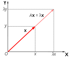
Illustration of a vector {$\mathbf{x}$} that satisfies {$A\mathbf{x} = \lambda\mathbf{x}. \;\; \mathbf{x}$} is simply rescaled (not rotated) by {$A$}. [image from Wikipedia]
All non-zero vectors {$\mathbf{v}$} that satisfy such an equation are called eigenvectors of {$A$}, and their respective {$\lambda$} are called eigenvalues. "Eigen" is a German term, meaning "own" (as in "my own" or "self") or characteristic" or "peculiar to", which is appropriate for eigenvectors and eigenvalues because to a great extent they describe the characteristics of the transformation that a matrix represents. In fact, for every real-valued, symmetric matrix we can even write the matrix entirely in terms of its eigenvalues and eigenvectors. Specifically, for an {$m \times m$} matrix {$A$} we can state {$A = V \Lambda V^T$}, where each column of {$V$} is an eigenvector of {$A$} and {$\Lambda$} is a diagonal matrix with the corresponding eigenvalues along its diagonal. This is called the eigendecomposition of the matrix.
If you want to find some function {$f(A)$} of a matrix {$A$}, e.g {$e^A$}, how would you do it?
Some functions are easy {$A^2$}. others not so. All are easy if {$A$} is a diagonal matrix -- just apply the function to each element of the diagonal. Similarly, to ask is a matrix is "positive", we could ask if all the elements of its diagonal are positive.
How do we do this for a general (or for now a general symmetric) matrix?
Answer: do an eigendecomposition. Find the solutions to {$A\mathbf{v_j} = \lambda_j\mathbf{v_j}$}, then assemble the eigenvectors {$\mathbf{v_j}$} into a matrix {$V$} and put the eigenvalues {$\lambda_j$} as elements on the diagonal of a matrix {$\Lambda$}, and then {$A = V \Lambda V^T$}.
Now we can apply all of our operations {$f()$} to the eigenvalues as if they were scalars!
In practice, most eigenvalue solvers use methods such as power iteration to compute eigenvalues. Let's see how that works by multiplying some arbitrary vector {$x$} repeatedly by a matrix {$A$}. What will {$A A A A A A A x$} approach? Answer: a constant times the eigenvalue corresponding to the largest eigenvalue {$\lambda_1$} How do we know? Answer: write {$x$} in terms of the basis vectors {$v_i$}, by projecting it on to each of them. {$x = \sum_i <x,v_i> v_i$}
How fast will it become "pure"? Each multiplication will increase the component of {$v_1$} relative to {$v_2$} by a factor of {$\lambda_1 / \lambda_2$}