Logistic
Logistic Regression
We saw how a generative classifier, the Naive Bayes model, works. It assumes some functional form for {$\hat{P}(X|Y)$}, {$\hat{P}(Y)$} and estimates parameters of P from training data. It then uses Bayes rule to calculate {$\hat{P}(Y|X=x)$}. In generative models, the computation of {$P(Y|X)$} is always indirect, through Bayes rule. Discriminative classifiers, such as Logistic Regression, instead assume some functional form for {$P(Y|X)$} and estimate parameters of {$P(Y|X)$} from training data. We first consider the simplest case of binary classification, {$y\in \{-1,1\}$}. The model uses the logistic function {$f(x)=1/(1+e^{-x})$} which transforms a real-valued input into a value between 0 and 1:
{$P(Y=1|\textbf{x},\textbf{w}) = \frac{1}{1+\exp\{-\sum_j w_j x_j\}} = \frac{1}{1+\exp\{-\textbf{w}^\top\textbf{x}\}} = \frac{1}{1+\exp\{-y\textbf{w}^\top\textbf{x}\}}$}
{$P(Y=-1|\textbf{x},\textbf{w}) = 1- P(Y=1|\textbf{x},\textbf{w}) = \frac{\exp\{-\textbf{w}^\top\textbf{x}\}}{1+\exp\{-\textbf{w}^\top\textbf{x}\}} = \frac{1}{1+\exp\{-y\textbf{w}^\top\textbf{x}\}}$}
or {$ log( \frac{ P(Y=1|\textbf{x},\textbf{w}) }{ P(Y=-1|\textbf{x},\textbf{w}) }) = \textbf{w}^\top\textbf{x} $}
The logistic (or sigmoid function) is equal to 0.5 when the argument is zero and tends to 0 for negative infinity and to 1 for positive infinity:
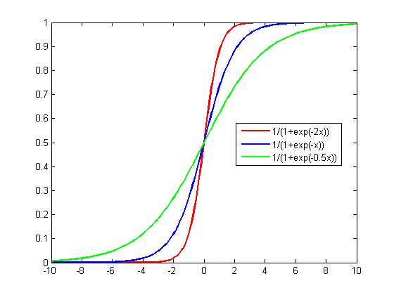
Logistic function
1-D Example
Consider a 1D problem, with positive class marked as pluses and negative as circles.
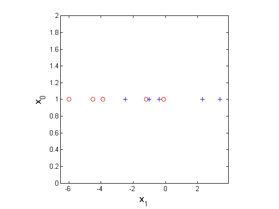
Classification dataset in 1D. Vertical axis is the constant feature {$X_{0} = 1$}
The log likelihood of the data {$\ell(\textbf{w})$} is:
{$ \log(P(D_Y | D_X,\textbf{w})) = \log\Bigg(\prod_i \frac{1}{1+\exp\{-y_i\textbf{w}^\top\textbf{x}_i\}}\Bigg) = -\sum_{i} \log (1+\exp\{-y_i\textbf{w}^\top\textbf{x}_i\})$}
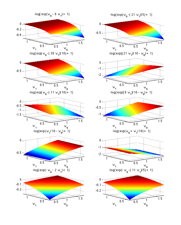
This log likelihood function is shown below in the space of the two parameters {$w_0$} and {$w_1$}, with the maximum at {$(w_0=1, w_1=0.7)$}.
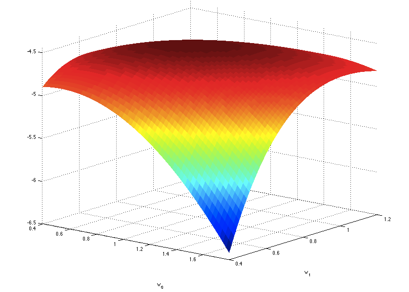
Log likelihood for dataset above
and here is a "heat map":
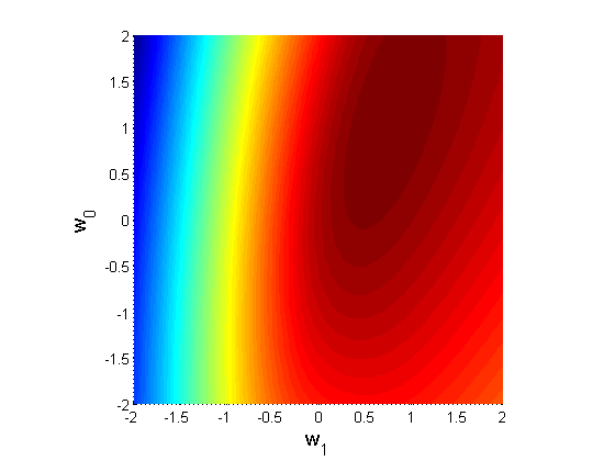
Log likelihood heat map for dataset above
Here are the plots of the contributions of each example to the objective above:
A plot of each example's contribution
The MLE solution is displayed below.
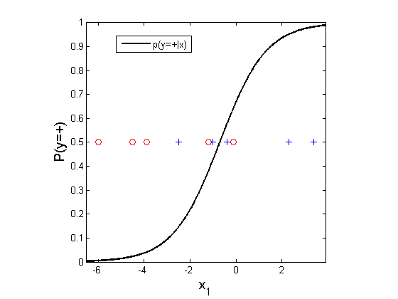
Learned logistic regression
2-D Example
Now consider a 2D problem, with positive class marked as pluses and negative as circles. In order to visualize the problem in 2D, we are not using the constant feature {$x_0$}.
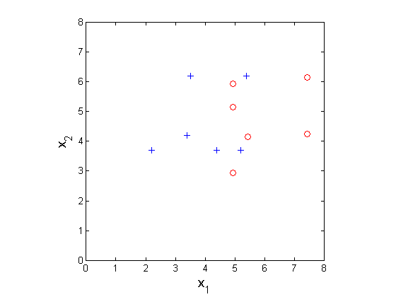
Classification dataset in 2 dimensions
The log likelihood of the data {$\ell(\textbf{w})$} is:
{$\log(P(D_Y | D_X,\textbf{w})) = \log\Bigg(\prod_i \frac{1}{1+\exp\{-y_i\textbf{w}^\top\textbf{x}_i\}}\Bigg) = -\sum_{i} \log (1+\exp\{-y_i\textbf{w}^\top\textbf{x}_i\})$}
This log likelihood function is shown below in the space of the two parameters {$w_1$} and {$w_2$}, with the maximum at (-0.81,0.81).
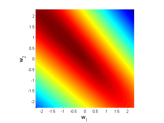
Log likelihood function heat map
The MLE solution is displayed below, where the red color indicates high probability of positive class. The black line shows the decision boundary learned by MLE.
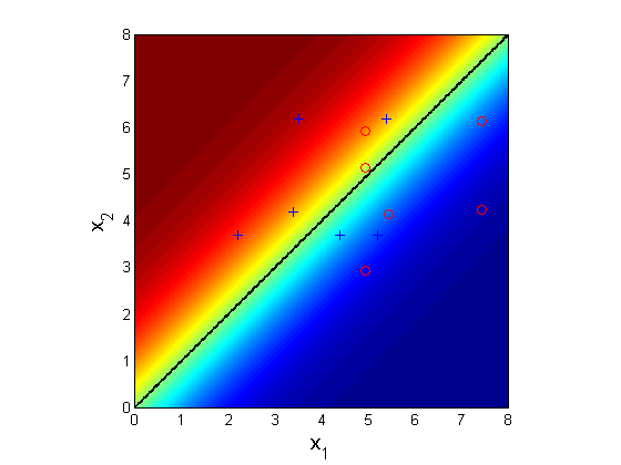
Learned logistic regression
Linear Decision Boundary
Why is the boundary linear? Consider the condition that holds at the boundary:
{$P(Y=1|\textbf{x},\textbf{w})=P(Y=-1|\textbf{x},\textbf{w}) \;\rightarrow\;\frac{1}{1+\exp\{-\textbf{w}^\top\textbf{x}\}} = \frac{\exp\{-\textbf{w}^\top\textbf{x}\}}{1+\exp\{-\textbf{w}^\top\textbf{x}\}} \;\rightarrow\; \textbf{w}^\top\textbf{x} = 0$}
For the toy problem above, the optimal {$\textbf{w}$} is (-0.81,0.81), so solving {$\textbf{w}^\top\textbf{x} = -0.81x_1+0.81x_2=0$} we get the line {$x_1 = x_2$}.
Computing MLE
Unfortunately, solving for the parameters is not "closed form", like it is Naive Bayes or for least squares regression. To find the MLE we will resort to iterative optimization. Luckily, the function we're trying to optimize is concave (concave downwards, or equivalently convex upwards), which means it has one global optimum (caveat: it may be at infinity). The simplest form of optimization is gradient ascent: start at some point, let's say {$\textbf{w}^0=0$} and climb up in steepest direction. The gradient of our objective is given by:
{$\nabla_{\textbf{w}}\;\ell(\textbf{w}) = \frac{\delta\log(P(D_Y | D_X,\textbf{w}))}{\delta\textbf{w}} = \sum_{i} \frac{y_i\textbf{x}_i\exp\{-y_i\textbf{w}^\top\textbf{x}_i\}}{1+\exp\{-y_i\textbf{w}^\top\textbf{x}_i\}} = \sum_{i} y_i\textbf{x}_i (1-P(y_i|\textbf{x}_i,\textbf{w}))$}
Gradient ascent update is (iterate until change is in parameters is smaller than some tolerance):
{$\textbf{w}^{t+1}= \textbf{w}^{t} + \eta_t\nabla_{\textbf{w}}\ell(\textbf{w})$}
where {$\eta_t>0$} is the update rate.
Computing MAP
Just like in regular regression, we assume a prior on the parameters {$\textbf{w}$} that we are trying to estimate. We will pick the simplest and most convenient one, the zero-mean Gaussian with a standard deviation {$\lambda$} for every parameter:
{$ w_j \sim \mathcal{N}(0,\lambda^2)\;\; {\rm so}\;\; P(\textbf{w}) = \prod_j \frac{1}{\lambda\sqrt{2\pi}} \exp\Bigg\{\frac{-w_j^2}{2\lambda^2}\Bigg\} $}
So to get the MAP we need:
{$ \arg\max_\textbf{w} \;\;\; \log P(\textbf{w} \mid D, \lambda) = \arg\max_\textbf{w} \left(\ell(\textbf{w}) + \log P(\textbf{w} \mid \lambda)\right) = \arg\max_\textbf{w} \left(\ell(\textbf{w}) - \frac{1}{2\lambda^2} \textbf{w}^\top\textbf{w} \right)$}
The gradient of the MAP objective is given by:
{$\nabla_{\textbf{w}}\;\log P(\textbf{w} \mid D, \lambda) = \sum_{i} y_i\textbf{x}_i (1-P(y_i|\textbf{x}_i,\textbf{w})) - \frac{1}{\lambda^2}\textbf{w}$}
Note the effect of the prior: it penalizes large values of {$\textbf{w}$}.
Multinomial Logistic Regression
Generalizing to the case when the outcome is not just binary, but has K classes, is simple. We simply have K-1 sets of weights, {$\textbf{w}_1,\ldots \textbf{w}_{K-1}$}, one for each class minus one, since the last one is redundant.
{$P(Y=k|\textbf{x},\textbf{w}) = \frac{\exp\{\textbf{w}_{k}^\top\textbf{x}\}}{1+\sum_{k'=1}^{K-1}\exp\{\textbf{w}_{k'}^\top\textbf{x}\}}, \;\;\;{\rm for }\;\;\; k = 1, \ldots, K-1$}
{$P(Y=K|\textbf{x},\textbf{w}) = \frac{1}{1+\sum_{k'=1}^{K-1}\exp\{\textbf{w}_{k'}^\top\textbf{x}\}}$}
When MAP estimation is used, it is also common to use a symmetric version, with all K sets of weights (even though one is redundant) since the prior is typically a zero-mean Gaussian, so singling out one of the classes as special (not having it's own weights) would introduce an unintended bias:
{$P(Y=k|\textbf{x},\textbf{w}) = \frac{\exp\{\textbf{w}_{k}^\top\textbf{x}\}}{\sum_{k'=1}^{K}\exp\{\textbf{w}_{k'}^\top\textbf{x}\}}, \;\;\;{\rm for }\;\;\; k = 1, \ldots, K$}
Naive Bayes vs. Logistic Regression
Let's consider the differences between the approaches:
| Model | Naive Bayes | Logistic Regression |
|---|---|---|
| Assumption | {$P(\textbf{X}|Y)$} is simple | {$P(Y|\textbf{X})$} is simple |
| Likelihood | Joint | Conditional |
| Objective | {$\sum_i \log P(y_i,\textbf{x}_i)$} | {$\sum_i \log P(y_i\mid\textbf{x}_i)$} |
| Estimation | Closed Form | Iterative (gradient, etc) |
| Decision Boundary | Quadratic/Linear (see below) | Linear |
| When to use | Very little data vs parameters | Enough data vs parameters |
Linear boundary for 2-class Gaussian Naive Bayes with shared variances
For Gaussian Naive Bayes, we typically estimate a separate variance for each feature j and each class k, {$\sigma_{jk}$}. However consider a simpler model where we assume the variances are shared, so there is one parameter per feature, {$\sigma_{j}$}. What this means is that the shape (the density contour ellipse) of the multivariate Gaussian for each class is the same. In this case the equation for Naive Bayes is exactly the same as for logistic regression, and the decision boundary is linear:
{$P(Y=1|X) = \frac{1}{1 + \exp\{w_0 + \textbf{w}^\top X\}}, \; {\rm for}\;\; {\rm some} \;\; w_0,\textbf{w}$}
Let's derive it:
{$ \begin{align*} P(Y=1|X) & = \frac{P(Y=1)P(X|Y=1)}{P(Y=1)P(X|Y=1)+P(Y=0)P(X|Y=0)}\\ & = \frac{1}{1+\frac{P(Y=0)P(X|Y=0)}{P(Y=1)P(X|Y=1)}}\\ & = \frac{1}{1+ \exp\Big(\log \frac{P(Y=0)P(X|Y=0)}{P(Y=1)P(X|Y=1)}\Big)} \end{align*} $}
Now let's plug in our definitions:
{$ \begin{align*} P(Y=1) & =\theta \\ P(X_j|Y=1) & = \frac{1}{\sigma_j\sqrt{2\pi}} \exp\Bigg\{\frac{-(X_j-\mu_{j1})^2}{2\sigma_j^2}\Bigg\}\\ P(X_j|Y=0) & = \frac{1}{\sigma_j\sqrt{2\pi}} \exp\Bigg\{\frac{-(X_j-\mu_{j0})^2}{2\sigma_j^2}\Bigg\} \end{align*} $}
We have:
{$ \begin{align*} & \log \frac{P(Y=0)P(X|Y=0)}{P(Y=1)P(X|Y=1)} \\ & = \log P(Y=0) + \log P(X|Y=0) - \log P(Y=1) - \log P(X|Y=1)\\ & = \log \frac{P(Y=0)}{P(Y=1)} +\sum_j\log\frac{P(X_j|Y=0)}{P(X_j|Y=1)} \\ & = \log \frac{1-\theta}{\theta} + \sum_j \frac{(\mu_{j0} - \mu_{j1})X_j}{\sigma_j^2} + \frac{\mu_{j1}^2 - \mu_{j0}^2}{2\sigma_j^2}\\ & = w_0 + \textbf{w}^\top X\end{align*} $}
Note that here we're using capital {$X$} and {$X_j$} to denote that these are random variables (and not to imply that they are matrices).