LocalLearning
The Supervised Learning Problem
Before we talk about any specific ML method, it's first useful to formally introduce some mathematical notation and formally discuss what a supervised machine learning algorithm does.
The first type of problem we will discuss in this class is supervised learning -- that is, learn a function to predict outputs from (input, output) examples. In general, we use {$X$} to represent the inputs to the problem, and {$Y$} to represent the outputs. Regardless of the nature of the input {$X$} (discrete, continuous, etc.), we can then distinguish problems by the domain of the output {$Y$}:
- Classification: {$Y \in \{0,1\}$} or {$Y \in \{-1,+1\}$}. Predicting whether or not a given input belongs to one of two classes, typically in terms of true or false, or positive or negative. (e.g., face detection).
- Regression: {$Y \in \mathbb{R}$}. Predicting a real number. (e.g., predicting gas prices).
- Multi-class Classification: {$Y \in \{1, \dots, K\}$}. Predicting which of {$K$} classes an input belongs to. (e.g., face recognition).
A critical concept in supervised learning is the training vs. testing data distinction. The learning process works like so:
- Training: A learner {$L$} is given a set of training data {$(x_1,y_1), \dots, (x_n, y_n)$} and allowed to perform computations on the training data to learn an output function {$h(x)$}.
- Testing: {$L$} is asked to generate predictions {$h(x_1), \dots, h(x_m)$} for a set of testing data. We can then compute an error metric or loss function to determine quantitatively if the learner correctly predicted the true outputs for the test examples. A common metric for classification tasks is the 0-1 loss, which is just the proportion of incorrect guesses:
{$loss_{01 error} = \frac{1}{m} \sum_{j=1}^m \mathbf{1}[h(x_j) \ne y_j] $}
Here are some important questions about this process: What happens if we use the same data for training and testing? Can we be confident about the algorithm's accuracy on new datasets? How can we train and test a learner if we only have a finite amount of collected data? More generally, how do we collect {$X$} and define {$Y$} for a given problem?
Now we are ready to move on to talking about a specific class of machine learning algorithms.
Local Learning
The class of learning methods we'll consider at first seem less like learning and more like pure memorization. In fact, one of the many names for local learning methods is memory-based learning, as well as instance-based, case-based, or distance-based. The idea is extremely simple: given a new example x, find the most similar training example(s) and predict a similar output. A boozy NN testimony by Alyosha.
The video below is a very nicely rendered illustration of this idea: nearest neighbor classification.

More generally, we will assume some measure of similarity or distance between examples and learn a local model, specific to the neighborhood of the new example.
Nearest Neighbor Methods
The nearest neighbor idea and local learning, in general, are not limited to classification, and many of the ideas can be more easily illustrated for regression. Consider the following one-dimensional regression problems:


Clearly, linear models do not capture the data well.
We can add more features, like higher order polynomial terms, or we can use a local approach, like nearest neighbors:
1-Nearest Neighbor Algorithm
- Given training data {$D=\{x_i,y_i\}$}, distance function {$d(\cdot,\cdot)$} and input {$x$}
- Find {$j = \arg\min_i d(x,x_i)$} and return {$y_j$}
Here are a few examples that illustrate the above algorithm with {$d(x,x_i) = |x-x_i|$} as x varies:
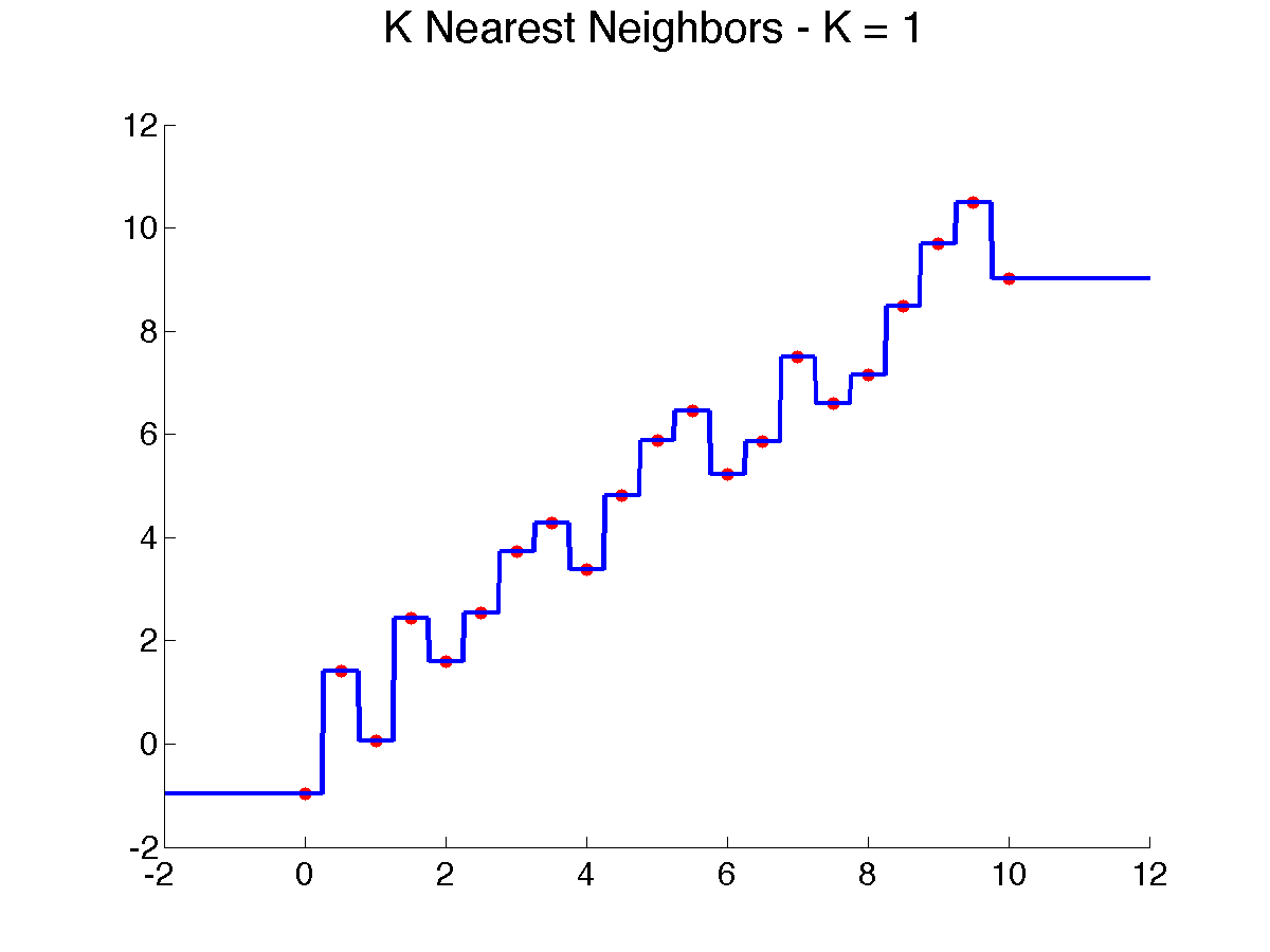
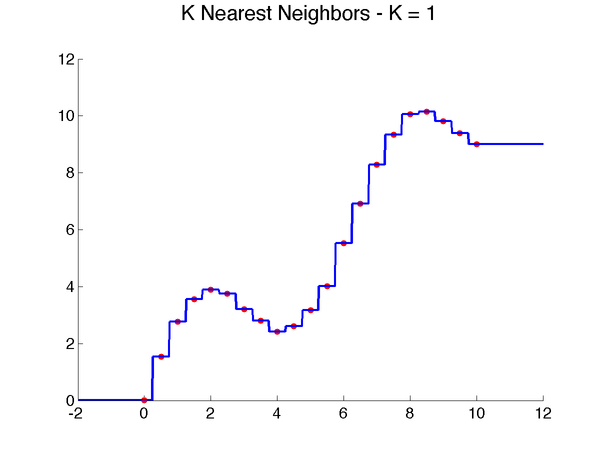
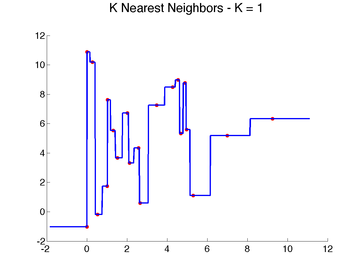
In one dimension, each training point will produce a horizontal segment that extends from half the distance to the point on the left to half the distance of the point on the right. These midway points are where the prediction changes. In higher dimension, if we use standard Euclidean distance (the one derived from the L2 norm) {$\|\mathbf{x}-\mathbf{x}_i\|_2$}, the regions where the closest training instance is the same will be polygonal. This tessellation of input space into the nearest neighbor cell is known in geometry as a Voronoi diagram. In 2D, it can be easily visualized (try the applet below, which allows you to move the points around!).

More generally, we can use an arbitrary distance function to define a nearest neighbor. (Note that every norm has a corresponding distance.) Some popular choices besides {$||\mathbf{x}-\mathbf{x}_i||_2$} include other norms: {$||\mathbf{x}-\mathbf{x}_i||_1$}, {$||\mathbf{x}-\mathbf{x}_i||_\infty $}. Below are the contours of {$L_2$}, {$L_1$} and {$L_\infty$} norms, respectively, where {$\mathbf{x}$} is placed at the center:
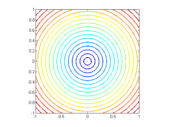 | 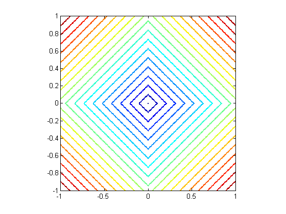 | 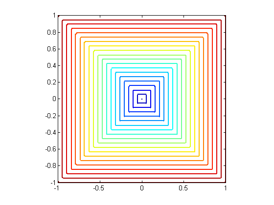 |
| {$L_{2} norm$} | {$L_{1} norm $} | {$L_{\inf} norm $} |
Their Voronoi diagrams are shaped quite differently. To see this, we plot the decision boundary for the three norms on a simple toy dataset below. The data comes from 2 classes, represented by a circle or a cross; any new points landing in the blue region is classified as a circle, and in the red classified as a cross. By changing the norm, we obtain dramatically different decision boundaries:


Non-parametric models
1-Nearest Neighbor algorithm is one of the simplest examples of a non-parametric method. Roughly speaking, in a non-parametric approach, the model structure is determined by the training data. The model usually still has some parameters, but their number or type grows with the data. Note that other algorithms we will discuss, such as decision trees, are also non-parametric, while linear regression or Naive Bayes are parametric. Non-parametric models are much more flexible and expressive than parametric ones, and thus overfitting is a major concern.
1-NN Consistency, Bias vs Variance
One important concept we will formally return to later is bias vs variance trade-off. For supervised learning, bias quantifies errors an algorithm makes because it simply cannot represent the complexity of the true label distribution. On the other hand, variance is errors the algorithm makes because it can represent too much and therefore tends to overfit the limited training samples. One nice property of non-parametric prediction algorithms is that because the complexity increases as the data increases, with enough data, non-parametric methods are able to model (nearly) anything and therefore achieve (close to) zero bias for any distribution.
An algorithm whose bias is zero as the number of examples grows to infinity for any distribution {$P(y|x)$} is called consistent. Under some reasonable regularity conditions on {$P(y|x)$}, 1-Nearest Neighbor is consistent. The problem is that the strict memorization aspect of 1-NN leads to a large variance for any finite sample size.
K-Nearest Neighbors
One way to reduce the variance is local averaging: instead of just one neighbor, find K and average their predictions.
K-Nearest Neighbors Algorithm
- Given training data {$D=\{\mathbf{x}_i,y_i\}$}, distance function {$d(\cdot,\cdot)$} and input {$\mathbf{x}$}
- Find {$\{ j_1 , \ldots,j_K\}$} closest examples with respect to {$d(\mathbf{x},\cdot)$}
- (regression) if {$y \in \mathbf{R}$}, return average: {$\frac{1}{K}\sum_{k=1}^{K} y_{j_k}$}
- (classification) if {$y \in \pm 1$}, return majority: {$sign(\sum_{k=1}^{K} y_{j_k})$}
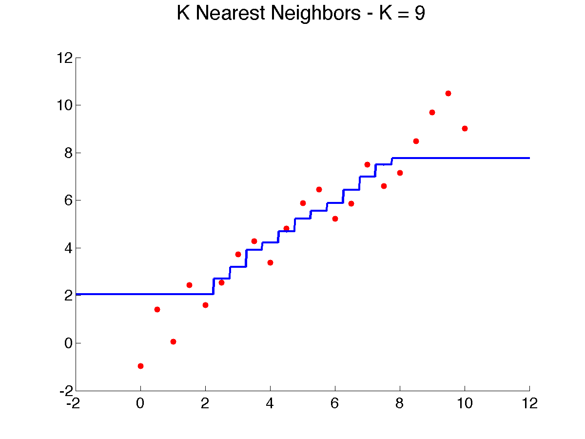
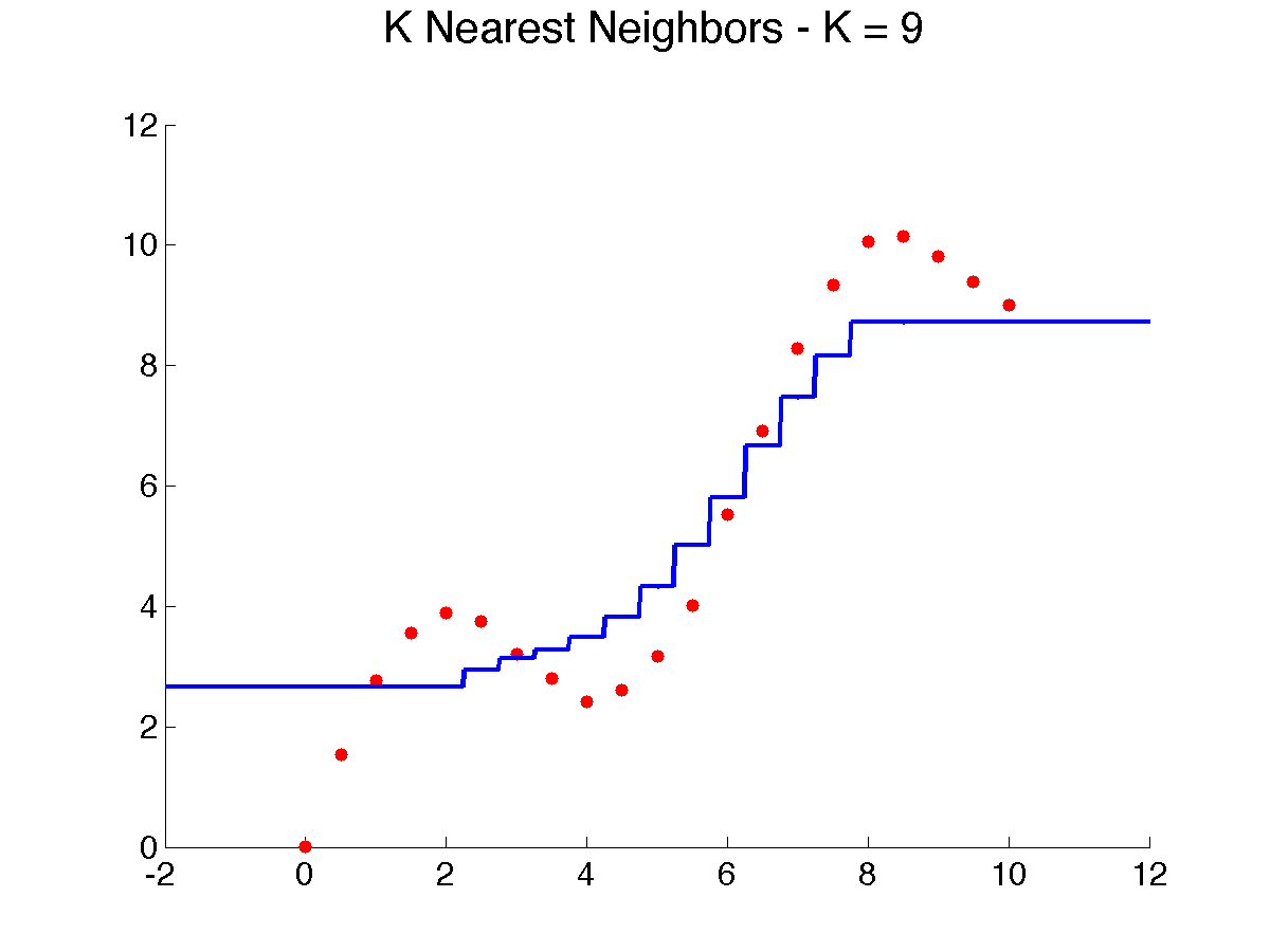
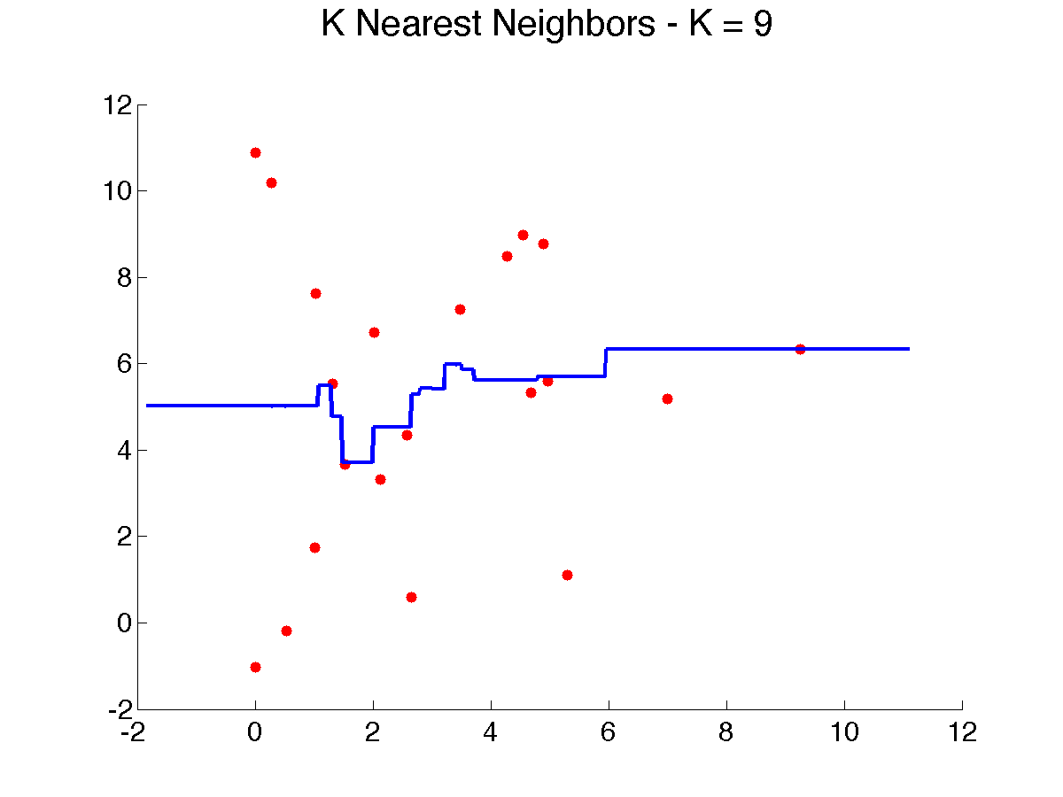
Here's a result of using 9 neighbors on our examples, which makes the prediction smoother, but still leaves several artifacts, especially near the edges:
Going back to our 2D toy dataset, we see we can achieve a "smoother" decision boundary by increasing {$K$} from 1 to 3:
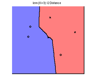
Note that we now misclassify one of the training points. This is an example of the bias-variance tradeoff. (We will return to this concept in later lectures.)
While local learning methods are very flexible and often very effective, they have some disadvantages:
- Expensive: need to remember (store) and search through all the training data for every prediction
- Curse-of-dimensionality: In high dimensions, all points are far from each other.
- Irrelevant features: If {$\mathbf{x}$} has too many irrelevant, noisy features,the distance function becomes useless.
Many methods generalize on k-nn, including k-means (covered later) and kernel regression (not covered) Back to Lectures