ICA
Independent Components Analysis (ICA)
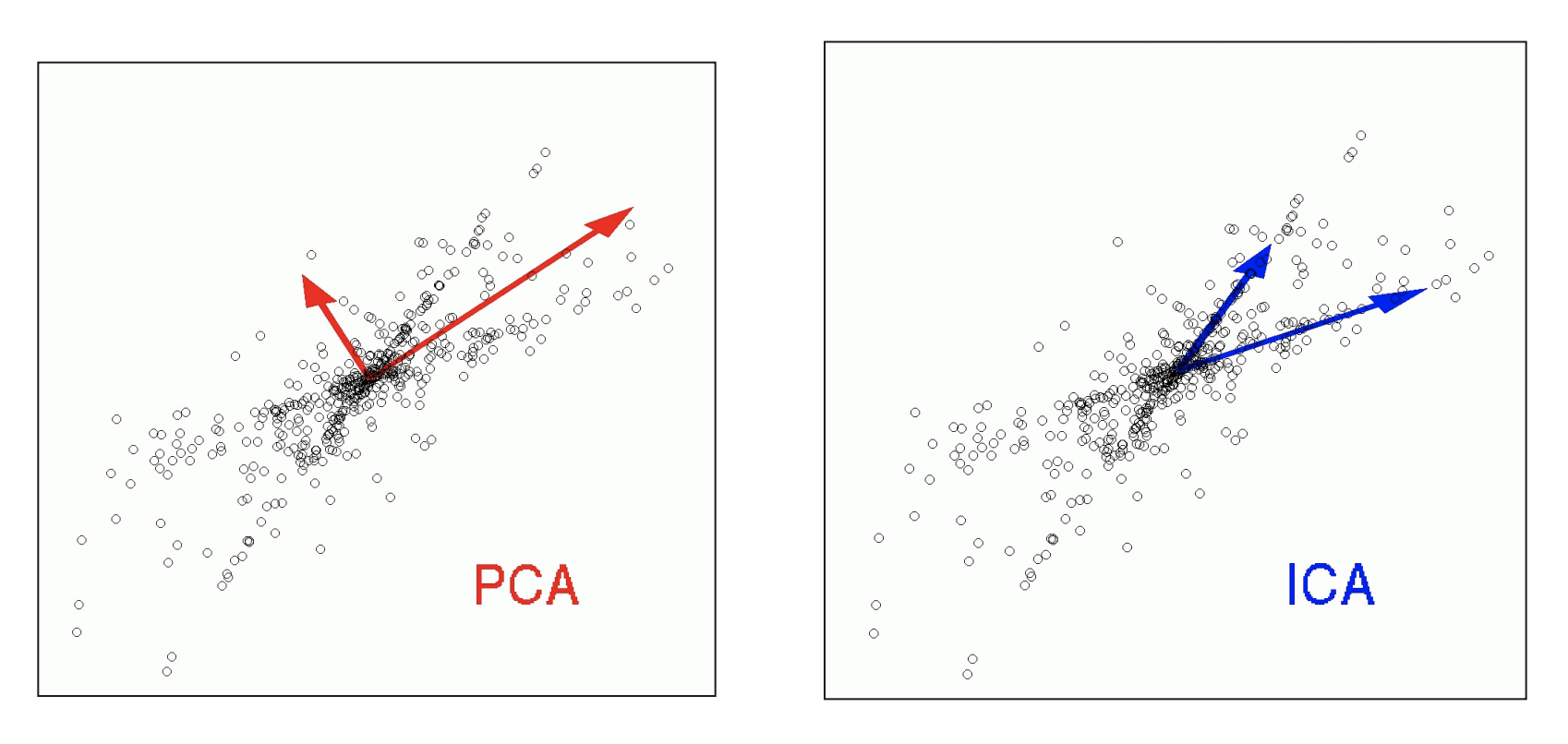
ICA is abstractly similar to PCA, but PCA tries to find a transformation of a matrix {$X$} to a new set of latent variables ("Principle component scores") {$Z$} such that the new latent variables are orthogonal, ICA finds sources {$S$} which are independent. (See, for example, the following nice figure from this side deck.
As with PCA, where we wrote {$ X \sim ZV^T$}, in ICA, we write {$S = XW $}, or {$X \sim SW^+ = (XW)W^+ $} and in Reconstruction ICA (the one we looked at), we try to minimize {$||X - SW^+||_F = ||X - (XW)W^+||_F$}, but instead of enforcing orthogonality, we try to make the different "sources" (the columns of {$S$}) to be "as independent" of each other as possible. (Equally common is to make the sources as non-Gaussian as possible.) There are over 100 different ICA algorithms, and they optimize many different criteria. We focus on one of these: minimizing the KL divergence (or equivalently, the mutual information) between the sources, {$KL(p(s_1,s_2,…s_m) | p(s_1)p(s_2) ...p(s_m))$}, where each of the {$m$} sources {$s_k$} is viewed as {$n$} observations from a probability distribution. Note that this is a definition of "as independent of each other as possible". If the sources were fully independent, then it would be the case that {$p(s_1,s_2,…s_m) = p(s_1)p(s_2) ...p(s_m)$}, and the KL-divergence would be zero.
In standard practice, the first step of ICA is to "whiten" the matrix {$X$} by multiplying it by the inverse square root of the covariance matrix: {$(X^TX)^{-1/2}$}.
There are a bunch of ways to actually estimate {$W$}. For example, one could pick some (non-Gaussian) distribution form, and estimate each {$p(s_k)$} to fit that probability distribution. One can also do non-parametric variations.