BNInference
Inference in Bayes nets
Inference in probabilistic models in general asks the following questions: given {$P(X_1,\ldots,X_m)$} and a set of observations {$e = \{X_i=x_i, X_j=x_j, \ldots\}$}, compute
- Marginals: {$P(X_k | e)$}
- Probability of evidence: {$P(e)$}
- Most probable explanation: {$\arg\max_x P(x|e)$}
- and many more
We will focus on the first question, {$P(X_k | e)$}.
Flu-Alergy-Sinus Example
Consider the Flu-Allergy-Sinus network
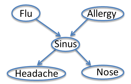
{$P(F,A,S,H,N)= P(F)P(A)P(S|F,A)P(H|S)P(N|S)$}
Let's compute {$P(F=t|N=t) \propto P(F=t,N=t)$}. We have
{$P(F,A,S,H,N)= P(F)P(A)P(S|F,A)P(H|S)P(N|S)$}
so:
{$ \; \begin{align*} P(F=t,N=t) & = \sum_{a,s,h} P(F=t,A=a,S=s,H=h,N=t) \\ & = \sum_{a,s,h} P(F=t)P(A=a)P(S=s|F=t,A=a)P(H=h|S=s)P(N=t|S=s) \end{align*} \; $}
We have a sum over {$2^3=8$} terms with 4 multiplies each. In general, we will have a sum with an exponential number of terms in the number of variables. General BN inference is unfortunately NP-hard. However, there are important and very useful special cases that exploit conditional independence and the distributive law: {$a(b+c) = ab + ac$}. And so:
{$ \; \begin{align*} P(F=t,N=t) & = \sum_{a,s} P(F=t)P(A=a)P(S=s|F=t,A=a)P(N=t|S=s)\sum_h P(H=h|S=s) \\ & = P(F=t)\sum_{a} P(A=a)\sum_s P(S=s|F=t,A=a)P(N=t|S=s) \end{align*} \; $}
Let's define an intermediate factor
{$ \; \begin{align*} g(A) & = \sum_s P(S=s|F=t,A=a)P(N=t|S=s) \\ & = P(N=t|F=t,A=a) \end{align*} \; $}
(which takes 2 multiplies and 1 add for each value a), then we have
{$P(F=t,N=t) = P(F=t)\sum_{a} P(A=a)g(A=a)$}
which takes 2 multiplies and 1 add, plus a final multiply. In general, we can often use the BN structure for exponential reduction in computation. The order in which we do the summations is absolutely critical.
Naive Bayes Example
Consider the naive Bayes example: {$P(Y,X_1,\ldots,X_m) = P(Y)\prod_i P(X_i|Y)$}.
{$ \; \begin{align*} P(X_1=x_1) & = \sum_{y,x_2,..,x_m} P(Y=y)\prod_{i=1}^m P(X_i=x_i|Y=y) \\ & = \sum_{x_2,..,x_m} \sum_y P(Y=y)\prod_{i=1}^m P(X_i=x_i|Y=y) \\ & = \sum_{x_2,..,x_m} g(X_1=x_1,\ldots,X_m=x_m) \end{align*} \; $}
Which is exponential. But, if we switch the order of summations:
{$ \; \begin{align*} P(X_1=x_1) & = \sum_{y,x_2,x,x_m} P(Y=y)\prod_{i=1}^m P(X_i=x_i|Y=y) \\ & = \sum_y P(Y=y)P(X_1=x_1|Y=y)\sum_{x_2}P(X_2=x_2|Y=y)\ldots\sum_{x_m}P(X_m=x_m|Y=y) \\ & = \sum_y P(Y=y)P(X_1=x_1|Y=y) \end{align*} \; $}
Variable Elimination
The generalization of this process of summing out of variables is the Variable Elimination Algorithm
Definition A factor {$f(\textbf{X})$} over variables {$X_i\in\textbf{X}$} is a function mapping joint assignments of {$\textbf{X}$} to non-negative reals.
The Variable Elimination Algorithm below uses factors to keep track of intermediate results. The invariant that is maintained throughout is the distribution over un-eliminated variables as a product of factors. In the beginning, the factors are just the original CPTs (modified by evidence). In the end, the only factor remaining is the distribution over the query variable.
Variable Elimination Algorithm
- Given a BN and a query {$P(X_k|e) \propto P(X_k,e)$}
- Initial set of factors is {$F = \{f_i(\textbf{X}_i) = P(X_i | Pa_{X_i})\}$}, so that {$P(X_1,\ldots,X_m) = \prod_i f_i(\textbf{X}_i)$}
- Instantiate evidence e in factors containing e by eliminating inconsistent entries
- Choose an ordering on variables,{$ (X_1, \ldots, X_m) $} (good heuristics exist, finding optimal is NP-hard)
- For i = 1 to m, If {$X_i \not \in \{X_k,e\}$}
- Collect factors {$f_1(\textbf{X}_1),\cdots,f_j(\textbf{X}_j)$} that include {$X_i$}, {$X_i \in \textbf{X}_1, \ldots ,\textbf{X}_j$}
- Generate a new factor by eliminating {$X_i$} from these factors {$f'(\textbf{X}') = \sum_{x_i} f_1(\textbf{X}_1) \times \ldots \times f_j(\textbf{X}_j)$}
- Remove {$f_1$}, {$\ldots,f_j$} from {$F$} and add {$f'$}
- Final remaining factor is {$f(X_k) = P(X_k,e)$}
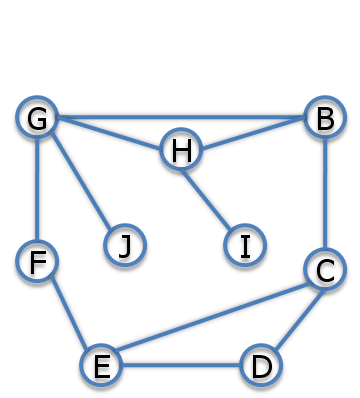
In the network below, we can choose an ordering such that inference is linear time! If we start from the leaves and work up to the roots: find topological order, eliminate variables in reverse order.
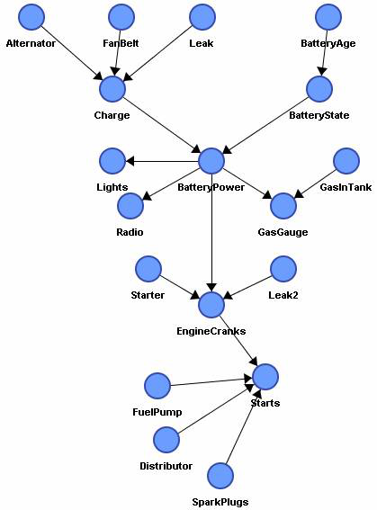
The complexity of VE depends critically on the ordering. In tree-BNS, the best ordering leads to linear time inference. In general BNs, the best ordering leads to an algorithm exponential in the number variables in a factor, called tree-width. Unfortunately, finding the best ordering in general is NP hard. There are many heuristics that work well though, like selecting the variable that creates the smallest new factor at every step.
A graphical view of the VE algorithm is quite intuitive. We can think of each factor as a clique of variables and edges between variables represent membership in some factor together. The first step (init) is called Moralization, where the directed graph is turned into an undirected graph and the parents are "married".
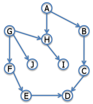
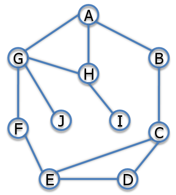
Each elimination step removes a variable and connects the neighbors. For example if we eliminate A, we multiply the factors that involve A, then sum out A and get a factor over B, G, and H, which means we need to add edges B-H and B-G:
The edges that are created by the elimination steps are called fill-in edges.
The algorithm above can be modified to compute the most probable explanation {$\arg\max P(X_1=x_1,\ldots, X_m=x_m|e)$} by changing the sum over the factors to a max (and keeping track of the maximizing entry). If we want to compute all marginals {$P(X_k,e)$} (for all k), there is a better algorithm that uses dynamic programming to compute them in just twice the cost of a single VE run, as we'll see when we discuss HMMs.