Auto-encoders
Auto-encoders learn a model that takes a vector {$\bf{x}$} as input, and predicts the same vector {$\bf{x}$} as output, trying to make the prediction as close as possible to the actual {$x$}, usually minimizing the Frobenius (L2) reconstruction error, {$||\bf{X}-\bf{\hat{X}}||_F$}. In the process, {$\bf{x}$} is mapped to a new feature set, or 'embedding', {$\bf{z} = f(\bf{x})$} which can then be used in other models. If {$f$} were invertable, then the reconstruction would be {$\hat{x} = f^{-1}(z) = f^{-1}(f(x))$}, but in general the inverse does not exist and is approximated by a pseudo-inverse: {$\hat{x} = f^+(z) = f^+(f(x))$}
Of course, one needs to do something to prevent overfitting, which in this case would lead to perfect reconstruction. Several approaches are used
- A 'bottleneck' such that the dimension of {$\bf{z}$} is less than that of {$\bf{x}$}
- Noise can be added to {$\bf{x}$}, making a denoising autoencoder
- Other regularization such as L1 or L2 penalties can be added to the model
- further penalties or constraints can be added to the model, such as forcing or encouraging orthogonality or independence (see below).
PCA as an auto-encoder
PCA, which we have covered in detail, is a linear autoencoder that forces the basis vectors for {$\bf{x}$} to be orthogonal, minimizes the usual Frobenius norm reconstruction error, and uses a bottleneck to avoid overfitting.
In PCA, we wrote {$ \hat{X} = ZV^T$}, where {$Z= XV$} are the "embeddings-- the ({$n*k$}) scores and ({$k*p$}) loadings {$V^T$} are orthonormal. Note the {$V^T$} and {$V$} are pseudo-inverses: {$V^TV=I$}
ICA
ICA, which we did not cover in detail, is a linear autoencoder that tries to make the encodings {$z_j$} be 'independent' of each other, for example making them have low mutual information.
In ICA, we write {$\hat{X} = SW^+ $} where {$S = XW$} are the "embeddings" or values of the "independent components".
The hope is that the {$s$} will be 'disentangled' in the sense that each element of {$s$} would represent an independent source such as a person talking or a car making noise or some other meaningful feature. This, of course, may or may not happen.
Denoising auto-encoders
Denoising auto-encoders simply use a neural network where the output is the feature vector {$x$} and the input is a "noisy" version of {$x$}, for example taking 10% of the pixels in an image and making them black.
This can be viewed as learning a neural net {$f(x)$}, which embeds {$x$} (with noise added, or a percentage of the pixes randomly blacked out) and a pseudo-inverse neual net {$f^+(z)$} that transforms {$z$} back to {$x$}:
{$\hat{x} = f^+(z) = f^+(f(x+\epsilon))$}
A similar idea is used in natural language processing, where one "masks" (removes), say, 10% of the words in a text and then uses the masked sentence as an input to predict the masked words.
Training autoencoders
One could simply train an end-to-end neural net to encode and decode feature vectors {$x$}. Usually one makes the encoder and decoder symmetric. If you take x, pass it through a neural layer {$A$} to get k1 outputs and then through another neural layer {$B$} to get k outputs (our {$z$}), then you would pass {$z$} through a pseudo-inverse layer {$B^+$} to get k1 outputs and through another layer {$A^+$} to reconstruct the p-dimensional input.
One can avoid doing back-propagation all the way through the autoencoder by sequentially training each layer. First, feed a noisy {$x$} through {$A$} and {$A^+$} and learn to reconstruct {$x$}. This gives you layers {$A$} and {$A^+$}. then take the k1-dimensional output of {$A$} and feed it through {$B$} and {$B^+$} to reconstruct it. Now we have a full encoder for {$x$}: the combined transformations {$A$} and {$B$}.
do the outside layer first, with {$A$} and {$A^+$}
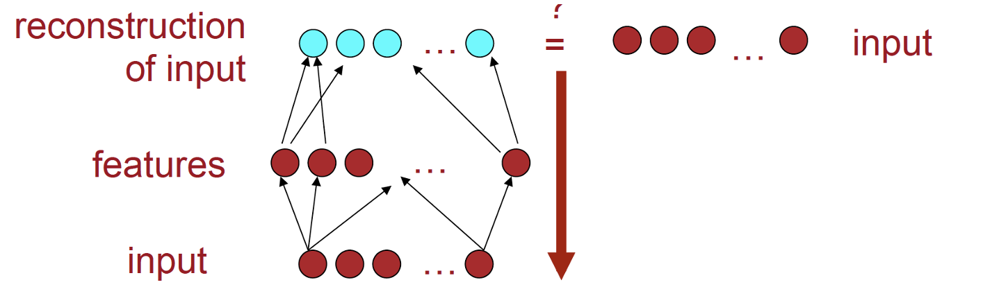
then learn the next layer in, with {$B$} and {$B^+$}
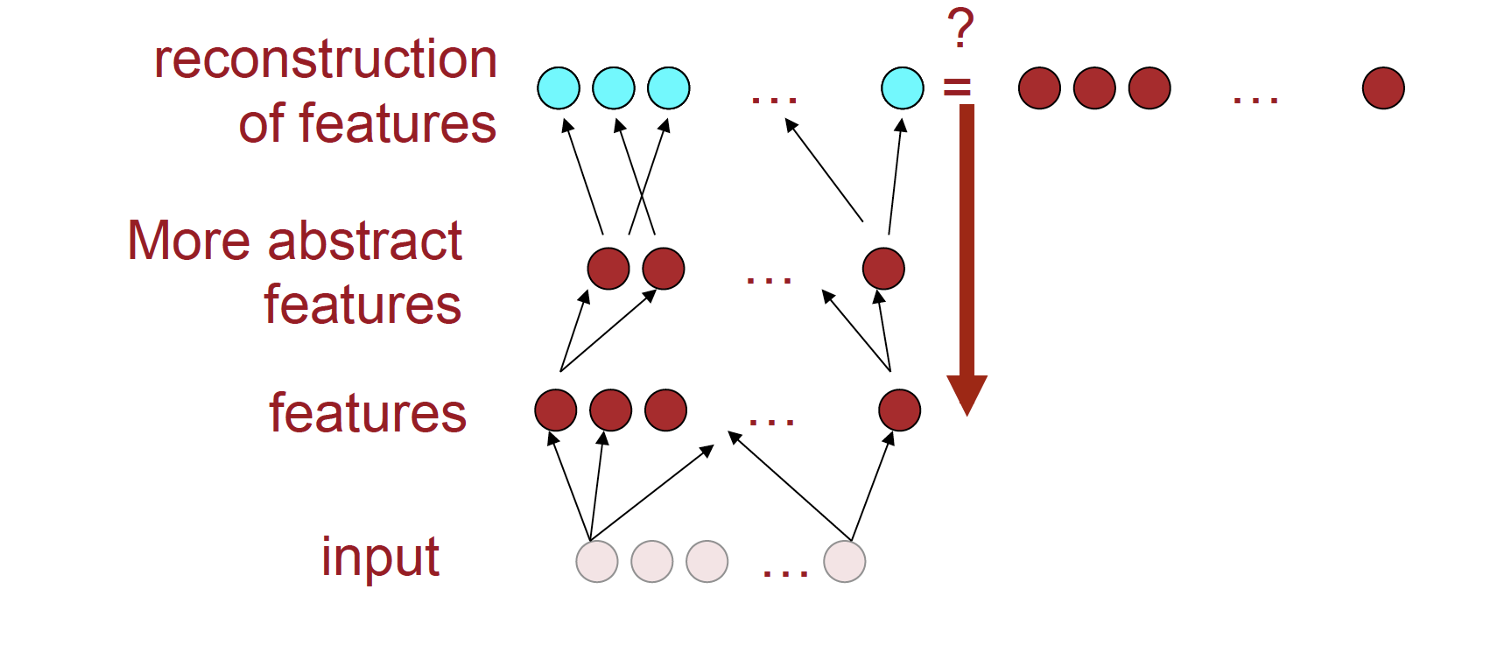
Images courtesy of Socher and Manning
Variational auto-encoders
The idea behind Variational auto-encoders is very much the same as with denoising ones, with an encoding and a decoding network, but instead of adding noise to the input, we use other constraints, such as bottlenecks or regularizers to prevent learning an identity reconstruction. One can either minimize the sum of squares (Frobenius) reconstruction error or the KL-divergence between the distribution of the inputs and their reconstructions.