• View
• Edit
• History
• Print

PCA

PCA does Dimensionality Reduction

Dimensionality reduction aims to change the representation of the data into a low-dimensional one while preserving the structure of the data. It is usually unsupervised. Its key uses are similar to clustering (e.g. K-Means and Mixtures of Gaussians clustering, which we will see later). In fact, we will eventually see that PCA, is like linear regression in having a probabilistic interpretation. Uses include

• Data visualization (2D plots of data make nice pictures)
• Pre-processing before further learning (fewer parameters to learn)

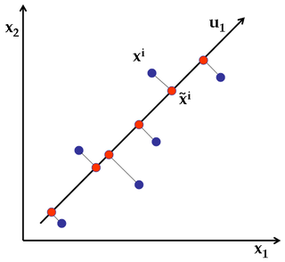
Principal Component Analysis is a linear dimensionality reduction technique: it transforms the data by a linear projection onto a lower-dimensional space that preserves as much data variation as possible. Here's a simple example of projecting 2D points into 1 dimension.

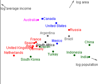
Here's a really nice applet illustration of the idea: projection of three dimensional information about countries into 2D.

Problem setup

Suppose our data consists, as usual, of n m-dimensional examples {$D = \mathbf{x}^1, \ldots, \mathbf{x}^n$} with {$\mathbf{x}^i \in \textbf{R}^m$}. We are looking for an orthonormal basis {$\mathbf{u}_1,\ldots,\mathbf{u}_k$} that defines our projection:

{$\mathbf{u}_i^\top \mathbf{u}_j = 0,\; \mathbf{u}_i^\top \mathbf{u}_i = 1$}

We center the data by subtracting the mean {$\mathbf{\overline x} = \frac{1}{n}\sum_i\mathbf{x}^i$} since the offset of the data is not relevant to the projection. Given a basis, a projected point is

{$ \mathbf{z}^i = \left( (\mathbf{x}^i-\mathbf{\overline x})^\top\mathbf{u}_1, \ldots,(\mathbf{x}^i-\mathbf{\overline x})^\top\mathbf{u}_k \right)$}

We can approximately reconstruct the original point from {$\mathbf{z}^i$} by the inverse mapping:

{$\mathbf{\hat x}^i = \mathbf{\overline x} + \sum_{j=1}^k z^i_j \mathbf{u}_j$}

Let the reconstruction or distortion error of our projection be standard squared error:

{$\textbf{Distortion:} \;\;\ \sum_{i=1}^n ||\mathbf{x}^i - \mathbf{\hat x}^i||^2_2 = \sum_{i=1}^n \sum_{j = 1}^m (x_j^i - \hat{x}_j^i)^2.$}

So just like in K-means, we're looking for a low-distortion representation of the data. PCA finds a k-basis that minimizes this distortion.

Distortion in Terms of Data Covariance

If we use {$k = m$} bases, the number of original dimensions, the reconstruction is perfect: the distortion is zero.

{$\mathbf{\hat x}^i = \mathbf{x}^i = \mathbf{\overline x} + \sum_{j=1}^m z^i_j \mathbf{u}_j$}

Rewriting distortion using this definition of {$\mathbf{x}^i$}, we have:

{$ \; \begin{align*} \textbf{Distortion}_k: \;\;\ \sum_{i=1}^n ||\mathbf{x}^i - \mathbf{\hat x}^i||_2^2 &= \sum_{i=1}^n ||\mathbf{\overline x} + \sum_{j=1}^m z^i_j \mathbf{u}_j - \mathbf{\overline x} - \sum_{j=1}^k z^i_j \mathbf{u}_j||_2^2 \\ &= \sum_{i=1}^n\left|\left|\sum_{j=k+1}^m z^i_j \mathbf{u}_j\right|\right|_2^2 \\ &= \sum_{i=1}^n \left(\sum_{j=k+1}^m z^i_j \mathbf{u}_j \right)^\top \left(\sum_{r=k+1}^m z^i_r \mathbf{u}_r \right) \\ &= \sum_{i=1}^n \sum_{j=k+1}^m \sum_{r=k+1}^m z^i_j z^i_r \mathbf{u}_j^\top\mathbf{u}_r. \end{align*} \; $}

Using orthonormality ({$\mathbf{u}_i^\top \mathbf{u}_j = 0,\; \mathbf{u}_i^\top \mathbf{u}_i = 1$}), we have:

{$\textbf{Distortion}_k:\;\;\ \sum_{i=1}^n \sum_{j=k+1}^m (z^i_j)^2$}

In words, the distortion is the sum of squares of full projection coefficients we discard.

We can express the distortion error in terms of the covariance of the features. Recall that {$z^i_j = (\mathbf{x}^i-\mathbf{\overline x})^\top\mathbf{u}_j$} and that the covariance matrix for the data is:

{$ \; \begin{align*} \Sigma & = \frac{1}{n}\sum_{i=1}^n (\mathbf{x}^i-\mathbf{\overline x}) (\mathbf{x}^i-\mathbf{\overline x})^\top \\ & = \frac{1}{n}\sum_{i = 1}^n \left[\begin{array}{ccc} (x_1^i - \overline{x}_1)(x_1^i -\overline{x}_1) & \ldots & (x_1^i - \overline{x}_1)(x_m^i - \overline{x}_m) \\ & \ddots & \\ (x_m^i - \overline{x}_m)(x_1^i - \overline{x}_1) & \ldots & (x_m^i - \overline{x}_m)(x_m^i - \overline{x}_m) \\ \end{array}\right] . \end{align*} \; $}

Then we have:

{$ \; \begin{align*} \textbf{Distortion}_k: & \sum_{i=1}^n \sum_{j=k+1}^m \mathbf{u}_j^\top(\mathbf{x}^i - \mathbf{\overline x})(\mathbf{x}^i-\mathbf{\overline x})^\top\mathbf{u}_j \\ & = \sum_{j=k+1}^m \mathbf{u}_j^\top \left(\sum_{i=1}^n (\mathbf{x}^i-\mathbf{\overline x}) (\mathbf{x}^i-\mathbf{\overline x})^\top \right) \mathbf{u}_j \\ & = n \sum_{j=k+1}^m \mathbf{u}_j^\top\Sigma \mathbf{u}_j \end{align*} \; $}

It can be shown that minimizing the distortion is equivalent to setting {$\mathbf{u}_j$}'s to be the eigenvectors of {$\Sigma$}. Here's a proof sketch. Consider the eigen-decomposition of {$\Sigma = \sum_{i=1}^m \lambda_i \mathbf{v}_i\mathbf{v}_i^\top$}. Suppose {$k=m-1$}, so we're only looking to throw away one basis function, {$\mathbf{u}_m$}. The distortion is

{$n \mathbf{u}_m^\top\Sigma \mathbf{u}_m = n \sum_{i=1}^m \lambda_i (\mathbf{v}_i^\top\mathbf{u}_m)^2.$}

To minimize this expression, (since {$\lambda_i$} are non-negative for a positive semi-definite matrix {$\Sigma$}), we need to put all the weight on the smallest eigenvalue: {$\mathbf{u}_m = \mathbf{v}_m$}. More formally, we can use Lagrangian formulation. Our problem is to minimize the {$\mathbf{u}_m^\top\Sigma \mathbf{u}_m$} such that {$\mathbf{u}_m$} is a unit vector:

{$\min_{\mathbf{u}_m} \mathbf{u}_m^\top\Sigma \mathbf{u}_m \;\;\;\;\textbf{s. t.}\; \; \mathbf{u}_m^\top\mathbf{u}_m = 1$}

The Lagrangian is {$L(\mathbf{u}_m,\lambda) = \mathbf{u}_m^\top\Sigma \mathbf{u}_m - \lambda (\mathbf{u}_m^\top\mathbf{u}_m - 1)$} Taking the derivative with respect to {$\mathbf{u}_m$} and setting it equal to zero, we get:

{$\Sigma \mathbf{u}_m = \lambda \mathbf{u}_m$}

Hence the stationary points of our problem are eigenvectors of {$\Sigma$}. Note that our problem has a non-convex constraint set, so there are multiple local minima. The smallest such minimum is the one with the smallest eigenvalue. The proof for the general case uses essentially this idea.

If we let {$\mathbf{u}_j$} be eigenvectors of {$\Sigma$}, then {$\Sigma\mathbf{u}_j = \lambda_j \mathbf{u}_j$} and {$\mathbf{u}_j^\top\Sigma\mathbf{u}_j = \lambda_j$}, the eigenvalue of {$\mathbf{u}_j$}. Hence,

{$\textbf{Distortion}_k: \;\;\ n\sum_{j=k+1}^m \lambda_j$}

Minimizing Distortion = Maximizing Variance

Instead of thinking of PCA as minimizing distortion, we can look at it from the opposite angle and think of it as maximizing the variance of the projected points. The variance of the projected points is

{$ \; \begin{align*} \textbf{Variance}_k: & \sum_{i=1}^n \sum_{j=1}^k (\mathbf{u}_j^\top\mathbf{x}^i-\mathbf{u}_j^\top\mathbf{\overline x})^2 \\ & = \sum_{j=1}^k \mathbf{u}_j^\top \left(\sum_{i=1}^n (\mathbf{x}^i-\mathbf{\overline x}) (\mathbf{x}^i-\mathbf{\overline x})^\top \right) \mathbf{u}_j \\ & = n \sum_{j=1}^k \mathbf{u}_j^\top\Sigma \mathbf{u}_j. \end{align*} \; $}

Maximizing the variance of projected points or minimizing the distortion of reconstruction leads to the same solution, using the eigenvectors of {$\Sigma$}. Note that when {$\mathbf{u}$}s are eigenvectors, we have:

{$\textbf{Variance}_k + \textbf{Distortion}_k = n\sum_{j=1}^m \lambda_j = n\textbf{trace}(\Sigma)$}

PCA Algorithm

PCA

• Given {$D = \mathbf{x}^1, \ldots, \mathbf{x}^n$}
• Compute {$\mathbf{\overline x} = \frac{1}{n}\sum_i\mathbf{x}^i$} and {$\Sigma = \frac{1}{n}\sum_{i=1}^n (\mathbf{x}^i-\mathbf{\overline x}) (\mathbf{x}^i-\mathbf{\overline x})^\top$}
• Find k eigenvectors of {$\Sigma$} with largest eigenvalues: {$\mathbf{u}_1,\ldots,\mathbf{u}_k$}, called loadings. (matlab calls these "coeff", as in "principal component coefficients")
• Project: {$ \mathbf{z}^i = \left( (\mathbf{x}^i-\mathbf{\overline x})^\top\mathbf{u}_1, \ldots,(\mathbf{x}^i-\mathbf{\overline x})^\top\mathbf{u}_k \right)$} called principal component scores. (matlab calls these "score")

Note that we only need the top {$k$} eigenvectors not all {$m$} of them, which is a lot faster to compute. In Matlab, the eigs function returns the top k eigenvectors of a matrix. In practice, good PCA code (like matlab's) will use SVD.

The eigenvectors form a set of basis vectors and the principal component scores are the weightings of each point {$x$} on the basis vectors. Alternatively, the scores are the points {$x$} transformed to a new coordinate system defined by the eigenvectors. The eigenvectors are called 'loadings' since they show, for each new point {$z$} how much it 'loads' on each of the original coordinates.

PCA can be also found using the SVD command, which avoids explicitly constructing {$\Sigma$}.

PCA via SVD

• Given {$D = \mathbf{x}^1, \ldots, \mathbf{x}^n$}
• Compute {$\mathbf{\overline x} = \frac{1}{n}\sum_i\mathbf{x}^i$} and stack the data into n-by-m matrix {$X_c$} where where the rows are {$\mathbf{x}^i - \mathbf{\overline x}$}
• Compute SVD of {$X_c = U S V^\top$}
• Take k rows of {$V^\top$} with largest singular values: {$\mathbf{v}_1,\ldots,\mathbf{v}_k$}, as principal loadings
• Project: {$ \mathbf{z}^i = \left( (\mathbf{x}^i-\mathbf{\overline x})^\top\mathbf{v}_1, \ldots,(\mathbf{x}^i-\mathbf{\overline x})^\top\mathbf{v}_k \right)$}

Formally, the SVD of a matrix {$A$} is just the decomposition of {$A$} into three other matrices, which we'll call {$U$}, {$S$}, and {$V$}. The dimensions of these matrices are given as subscripts in the formula below:

{$\textbf{SVD}:\;\;\; A_{n \times m} = U_{n \times n}S_{n \times m}V^T_{m \times m}.$}

The columns of {$U$} are orthonormal eigenvectors of {$AA^T$}. The columns of {$V$} are orthonormal eigenvectors of {$A^TA$}. The matrix {$S$} is diagonal, with the square roots of the eigenvalues from {$U$} (or {$V$}; the eigenvalues of {$A^TA$} are the same as those of {$AA^T$}) in descending order. These eigenvalues are called the singular values of {$A$}. For a proof that such a decomposition always exists, check out this SVD tutorial.

The key reason we would prefer to do PCA through SVD is that it is possible to compute the SVD of {$X_c$} without ever forming the matrix {$\Sigma$} matrix. Forming the {$\Sigma$} matrix and computing its eigenvalues is computationally expensive above can lead to numerical instabilities. There are ways to compute the {$USV^T$} decomposition of SVD that have better numerical guarantees, such as the power method "randomized SVD" described last class.

SVD is a useful technique in many other settings also. For example, you might find it useful when working on the project data to try latent semantic indexing. This is a technique that computes the SVD of a matrix where each column represents a document and each row represents a particular word. After SVD, each row in the {$U$} matrix represents the word with a "low dimensional vector". Words that are related (i.e. that tend to show up in the same document) will have similar vector representations. For example, if our original set of words was [hospital nurse doctor notebook Batman], hospital, nurse, and doctor would all be closer to each other than to notebook or Batman. Similary, one can compute eigenwords by taking the SVD between words and their contexts. If one uses the words before and after each target words as context, words that are "similar" are close - i.e. nurse and doctor would be similar, but not hospital. Examples here.

Eigenfaces

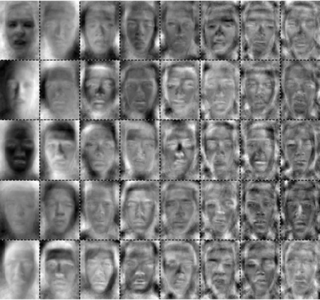
Suppose we had a set of face images as input data for some learning task. We could use each pixel in an image as an individual feature. But this is a lot of features. Most likely we could get better performance on the test set using fewer, more generalizable features. PCA gives us a way to directly reduce and generalize the feature space. Here's an example of how to do this in MATLAB: Eigenfaces.m.

Here is an example where we applied PCA to a set of face images:

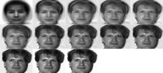
And here is an example of reconstruction [from Turk and Pentland, 91] using different numbers of bases.

Choosing the Number of Principal Components

Unlike in K-means or Gaussian mixtures, we can compute all the eigenvectors (or singular vectors) at once and then choose {$k$} appropriately. Often, {$k$} is chosen based on computational needs, to minimize memory or runtime. We can use the eigenvalue spectrum as a guide to good values of {$k$}. If the values drop off quickly after certain {$k$}, then very little is lost by not including later components.

Probabilistic Interpretation

PCA can be re-formulated in a probabilistic framework as a latent variable model with continuous latent variables. Bishop Chapter 12.2 has a full account of the approach, but the basic idea is to define a Gaussian latent variable {$\mathbf{z} \sim N(0,I)$} of dimension {$k$} and let {$p(\mathbf{x}|\mathbf{z}) = N(\mathbf{W}\mathbf{z}+\mu,\sigma^2I)$}, where {$\mathbf{W}$} is a m-by-k matrix. Maximum likelihood estimation of {$\mu,\mathbf{W}$} (as {$\sigma \rightarrow 0$}) leads to setting {$\mathbf{W}$} to be the eigenvectors of {$\Sigma$}, up to an arbitrary rotation.

Random Projections

In some cases, we want to reduce the dimensionality of a large amount of data or data with many, many dimensions. Performing PCA may be too costly (both in time and memory) in these cases. An alternative approach is to use random projections. The procedure for this is as follows:

Random Projections

• Given {$D = \mathbf{x}^1, \ldots, \mathbf{x}^n$}, stack the data into an {$n \times m$} matrix {$X$}
• Form a random {$m \times k$} matrix {$R$} by drawing each entry {$\sim \mathcal{N}(0, 1)$} and then normalizing the columns to have unit length
• Project: Compute the product {$XR$}

This will not yield the optimal basis we get with PCA, but it will be faster and there are theoretical results (take a look at the Johnson-Lindenstrauss lemma if you're curious) proving it is not too far from the PCA result as long as {$k$} is large enough.

Mean Subtraction

If we have data that is sparse in the original feature space, then subtracting the data mean, {$\mathbf{\overline x}$}, will make the data matrix {$X$} non-sparse and thus perhaps intractible to work with (it will take up too much memory). While you could just move from PCA to the random projection approach in order to get around this difficulty, it is also possible to simply run PCA without doing the mean subtraction step. Assuming the mean of the data is larger than the actual meaningful variance of the data, then this mean value would simply be captured by the first eigenvector. So, you could get the top {$k + 1$} eigenvectors and throw away the topmost, using the rest as your loading vectors.

Back to Lectures