VCDim

VC dimension examples

Recall that to prove the VC-dim of this class is some value {$d$}, we need to show two things:

There exists a set {$S$} of size {$d$} shattered by {$\mathcal{H}$}.
There does not exist a set {$S$} of size {$d+1$} shattered by {$\mathcal{H}$}.

Decision trees

What is the VC dimension of a 3-node decision tree in one dimension?

(:ans:) Each node deﬁnes a new splitting threshold on the data. Three thresholds deﬁne at most 4 regions on the axis, so the VC dimension is 4. (:ansend:)

What about a 7-node tree in one dimension?

(:ans:) Using the same reasoning as in the 3-node case, VC dimension in this case is 8. (:ansend:)

Origin-centered circles and spheres

What is the VC dimension of an origin-centered circle (2D) {$f(\mathbf{x}) = sign(a \mathbf{x}^\top\mathbf{x} + b)$}?

(:ans:) The VC dimension is 2. With any set of three points, they will be at some radii {$r_1 \leq r_2 \leq r_3$} from the origin, and no function {$f$} will be able to label the points at {$r_1$} and {$r_3$} with {$+1$} while labeling the point at {$r_2$} with {$-1$}. (The opposite labeling also cannot be achieved.) Thus, no set of three points is shatterable by origin-centered circles, making the VC dimension just 2. (:ansend:)

What about an origin-centered sphere (3D)?

(:ans:) The VC dimension in this case is also 2. The same reasoning as for the 2D case applies. (:ansend:)

Semi-circles

Suppose we were interested in using semi-circles as classifiers. That is, classifiers shaped like so:

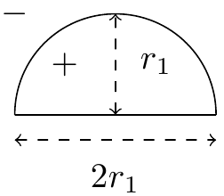
Points inside the semi-circle are labeled {$+1$} and those outside are labeled {$-1$}. Any rotated or scaled versions of the above drawing are also valid semi-circles. For example:

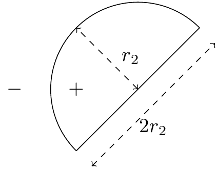
Which of the following conﬁgurations of 4 points can a semi-circle classifier shatter?

(:ans:) (a) and (b) are shatterable. For (c), the central point cannot be labeled {$-1$} while the other three points are labeled {$+1$}. (Keep in mind that for the hypothesis class we're considering, the interior of the semi-circle must take on label {$+1$}, not {$-1$}.) (:ansend:)

What about these conﬁgurations of 5 points?

(:ans:) Neither of the above sets are shatterable. For both sets, one labeling semicircles cannot achieve is shown below: (:ansend:)

Axis-aligned hyperplanes

What is the VC dimension of an axis-aligned hyperplane in two dimensions? Keep in mind that the formal deﬁnition of an axis-aligned hyperplane in two dimensions is {$f(\mathbf{x}) = sign(ax_c + b)$}, where {$c$} is either 1 or 2. That is, if the dimensions are {$x_1$} and {$x_2$}, then the hyperplane can be any line that is parallel to the {$x_1$} axis or the {$x_2$} axis. Hint: VC dimension is at most 3, since we know the VC dimension of general (non-axis-aligned) hyperplanes in {$n$} dimensions is {$n + 1$}.

(:ans:) The VC dimension is 3. An example of a shatterable set of three points is (0,0), (1,2), and (2,1). Invoking the upper bound of {$n + 1$}, 3 is the max size for a shatterable set. (:ansend:)

What about an axis-aligned hyperplane in three dimensions?

(:ans:) The VC dimension is 4. An example of a shatterable set of four points is (0,0,-1), (2,1,0), (-1,2,1) and (1,-1,2). Again invoking the upper bound of {$n + 1$}, 4 is the max size for a shatterable set. (:ansend:)

Monotone boolean conjunctions of literals

For this example, we'll consider binary classification as in many of the previous examples, but instead of {$y \in \{-1,+1\}$} we'll use {$y \in \{0,1\}$} because it will make notation simpler here. Let's look at the class of monotone boolean conjunctions of literals over {$\{ 0 , 1\}^m$}. (Monotone means the conjunctions do not contain negations.) In other words, the inputs are binary vectors of length {$m$}: {$x = x_1 x_2 x_3 \dots x_m$}, and classifiers take the form of either constants (like a conjunction of 0 literals):

{$h(x) = 1$} {$h(x) = 0$}

or else they have the form:

{$conjunction, h(x) = \bigwedge_{i \in S} x_i ,$}

where {${} S \subseteq \{1, \dots, m\}$} indicates which subset of the features are used. For example, the hypothesis {$h(x) = x_1 \wedge x_3$} returns {$+1$} if the first feature is {$1$} and the third feature is {$1$}, and {$0$} otherwise.

Prove the following claim: {$VC(\mathcal{H})$} is {$m$}.

Proof:

Let's show (1) first, that {$VC(\mathcal{H}) \ge m$}. We can do this by finding a set of points in {$m$} dimensions such that all possible labelings of these points can be achieved by monotone boolean conjunctions of literals. Consider arranging the {$m$} points {$x^{(1)}, \ldots, x^{(m)}$} such that:

{$x^{(j)}_i = \left\{ \begin{array}{cc} 0 & \;\textrm{if}\; j = i \\ 1 & \;\textrm{otherwise} \end{array} \right. $}

First, note that we can achieve the all 1s labeling for this set of points just by using the constant classifier {$h(x) = 1$}. To achieve a labeling where just one point {$x^{(i)}$} is labeled zero, we can use the classifier {$h(x) = x_i$}. (There are {$m$} such labelings, one for each of {$i = 1, \ldots, m$}.) To achieve a labeling where just two points {$x^{(i)}$} and {$x^{(j)}$} are labeled zero, we can use the classifier {$h(x) = x_i \wedge x_j$}. Extrapolating, to achieve the labelings with {$k \leq m$} zeros we can use the classifiers that are conjunctions of {$k$} literals. Therefore, we have shown that {$\mathcal{H}$} can give any labeling to these {$m$} points, meaning {$VC(\mathcal{H}) \ge m$}.

Now let's show (2), that {$VC(\mathcal{H}) \leq m$}. We can do this using a proof by contradiction. Suppose {$\mathcal{H}$} could shatter {$m+1$} points. Then for each point {$x^{(i)}$} there would be some conjunction {$c^{(i)}$} that labels this point 0 and all other points 1. Further, in this conjunction there must be some literal {$x^{(i)}_{f(i)}$} such that:

{$x^{(i)}_{f(i)} = 0\;\;\;\; $}

where the function {$f$} here just indicates a mapping from the datapoint index to the index of a zero literal within that datapoint. Since there are {$m+1$} points but only {$m$} literals, we have that one literal must occur at least twice in the set {$\{x_{f(1)}, \ldots, x_{f(m+1)}\}$}. Without loss of generality, suppose {$x_{f(1)} = x_{f(2)}$}. Then {$x^{(1)}_{f(1)}$} is 0 (corresponding to the point {$x^{(1)}$}) and {$x^{(2)}_{f(1)}$} is 0 (corresponding to the point {$x^{(2)}$}). But then {$c^{(1)}$} is 0 for both {$x^{(1)}$} and {$x^{(2)}$}. This is a contradiction, because our initial assumption was that {$c^{(1)}$} is only 0 for {$x^{(1)}$}. Thus, we have shown that {$\mthcal{H}$} cannot shatter any set of {$m+1$} points, so {$VC(H) \leq m$}.

References: Exact VC-Dimension of Boolean Monomials

Upper bounding VC dimension

Suppose we have a ﬁnite hypothesis space {$\mathcal{H}$} with {$|\mathcal{H}|$} unique classifiers. Knowing nothing else about {$\mathcal{H}$}, what is the tightest upper bound you can give on its VC dimension? Hint: Write an expression in terms of {$|\mathcal{H}|$}, as in {$VC(\mathcal{H}) \leq f(|\mathcal{H}|)$}, where {$f$} is the function you need to supply.

(:ans:) To shatter {$m$} points requires {$2^m$} labellings, so {$|\mathcal{H}| \geq 2^m$} would be necessary. Solving for {$m$} in this expression, we arrive at the upper bound {$VC(\mathcal{H}) = m \leq log_2 |\mathcal{H}|$}. (:ansend:)

Hyperplanes (revisited)

During the lecture we mensioned that "in general, we can show the VC dimension of hyperplanes in {$m$} dimensions is {$m+1$}".

Proof: Let {$\mathcal H$} be the set of hyperplanes in {$m$} dimensions. First, we show that there exists a set {$S$} of {$m+1$} points {$\in \mathbb R^m$} shattered by {$\mathcal H$}.

Suppose {$S = \{x_1, \hdots, x_m, x_{m+1}\}$}, where {$x_i$} is a point {$\in \mathbb R^m$}, and our hyperplane is represented as {$y=w^{\top}x+w_0$}. Let {$\ y_1, \hdots, y_m, y_{m+1}$} be any set of labels assigned to the {$m+1$} points and construct the following linear system:

{$w^{\top}x_1+w_0=y_1 $} {$w^{\top}x_2+w_0=y_2 $} {$\hdots $} {$w^{\top}x_{m+1}+w_0=y_{m+1}$}.

Notice that the above linear system as having {$m+1$} variables {$\ w_0, \hdots, w_m$} and {$m+1$} equations, hence it must have a solution as long as {$S$} satisfies the condition that {$(1, x_1), \hdots, (1, x_m), (1, x_{m+1})$} are linearly independent.

Hence by choosing {$S$} s.t. the matrix {$\left( \begin{array}{cc} 1 & x_1 \\ \vdots & \vdots \\ 1 & x_{m+1} \end{array} \right) $} is full-rank, we can always solve for a {$m$}-dimensional hyperplane with bias term that separates the {$m+1$} points in {$S$}. Since {{$\ y_1, \hdots, y_m, y_{m+1}$}} can be any set of labels, the {$m$}-dimensional hyperplane shatters the {$m+1$} points in {$S$}.

Secondly, we show that there exists no set {$S'$} of {$m+2$} points can be shattered by {$\mathcal{H}$}.

Suppose to the contrary that {$S'=\{x_1, \hdots, x_{m+1}, x_{m+2}\}$} can be shattered. This implies that there exist {$2^{m+2}$} weight vectors {$w^{(1)}, \hdots, w^{(2^{m+2})}$} such that the matrix of inner products denoted by {$z_{i,j}=x_i^{\top}w^{(j)}$} has columns with all possible combination of signs (note here {$x_i$} contains the constant feature and {$w^{(j)}$} contains the bias term). We use {$A$} to denote this matrix and

{$A=\left( \begin{array}{ccc} z_{1,1} & \hdots & z_{1,2^{m+2}} \\ \vdots & \hdots & \vdots \\ z_{m+2,1} & \hdots & x_{m+2, 2^{m+2}} \end{array} \right)\end{array} \right)\ s.t.\ sign(A)=\left( \begin{array}{ccccc} - & - & \hdots & - & + \\ - & \dot & \hdots & \dot & + \\ \vdots & \vdots & \hdots & \vdots & \vdots \\ - & + & \hdots & + & + \end{array} \right)$}.

Then the rows of {$A$} are linearly independent because there exists a column of {$A$} with the same signs which does not sum to zero hence there are no constants {$c_1, c_2, \hdots, c_{m+2}$} such that {$\sum_{i=1}^{m+2}c_iz_{i, :}=0$} . However, notice that row {$i$} of {$A$} can be written as {$x_i^{\top}W$} where {$W=[w^{(1)}, \hdots, w^{(2^{m+2})}]$}. By linear algebra knowledge we know that {$m+2$} vectors {$\in \mathbb R^{m+1}$}, are always linearly dependent (i.e. {$x_1^{\top}, \hdots, {$x_{m+2}^{\top}$} are linearly dependent). Hence {$x_1^{\top}W, \hdots, {$x_{m+2}^{\top}W$} should also be linearly dependent, which results in a contradiction.

This contradiction proves that there are no {$m+2$} points {$\in \mathbb R^m$} which can be shattered by hyperplanes in {$m$} dimension. Thus, the VC dimension of {$\mathcal{H}$} is {$m+1$}.

Note: the argument can also be proved by induction, which is left as an exercise.

Perceptron convergence

First, take a look at the lecture notes for the convergence proof.

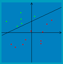
Then, check out this perceptron applet to gain some intuition about the algorithm. If you try it for separable data, you should notice that it works well in the sense that it converges relatively quickly on a separating line. However, keep in mind that this line will likely not have the nice max-margin property we get from SVMs. For example, the line below is the one the perceptron algorithm chooses for this separable dataset:

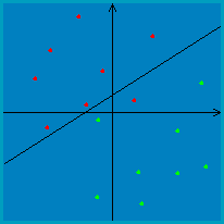
If you try running the perceptron applet for non-separable data, it should become apparent that some additional machinery is necessary in order to make the algorithm converge. That is, you will notice that the perceptron algorithm will oscillate back and forth between several different classifiers when the data is non-separable. For instance, for the example data shown below, the algorithm oscillates back and forth between classifiers like these two:

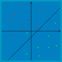
In practice, there are two ways we can deal with this:

Choose a small learning rate: Instead of updating {$\mathbf{w}_{t+1} = \mathbf{w}_t + y_t\mathbf{x}_t$} we could use a more conservative update formula with a learning rate parameter {$\eta \in (0, 1]$} so that {$\mathbf{w}_{t+1} = \mathbf{w}_t + \eta y_t\mathbf{x}_t$}. The smaller the value of {$\eta$}, the smaller the impact of a misclassified point on {$\mathbf{w}$}. While this won't entirely eliminate the oscillating behavior, it will make the oscillations smaller. That is, the classifiers oscillated between will be more similar to each other.
A more complete solution to the problem is the averaged perceptron algorithm. This is a modification to the perceptron algorithm that stores an averaged weight vector and makes final predictions based on this averaged vector. That is, we let each weight be the average of its values across all iterations. To implement this, you can simply use an auxiliary vector {$\mathbf{s}$} to store a running sum of {$\mathbf{w_t}$} and in the end divide {$\mathbf{s}$} by the total number of perceptron iterations run, {$T$}.