• View
• Edit
• History
• Print

OldExamqQuestions

Variable elimination: a numerical example

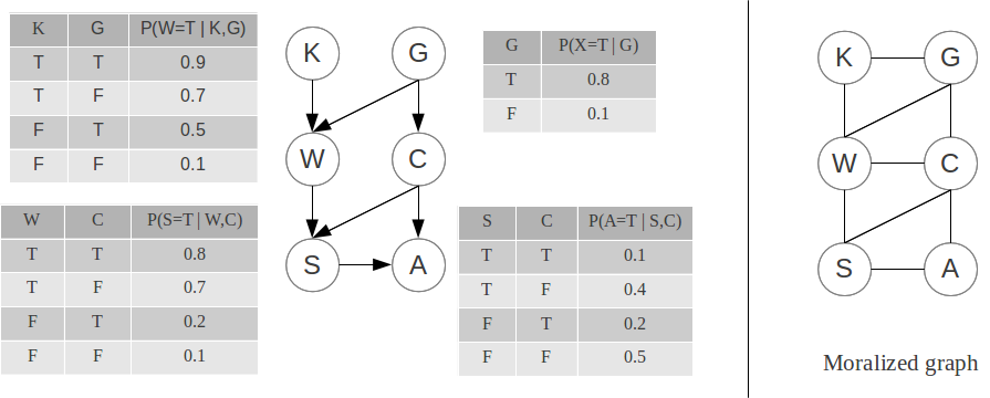
Consider the following Bayes net, modeling the behavior of a group of students and their professor. The variables are the following:

• K is true when the professor is knowledgeable,
• G is true when the professor is kind and generous,
• W is true when most of the students work hard,
• C is true when the professor gives candy bars to successful students,
• S is true when most students succeed on the final exam, and
• A is true when an alarming proportion of students develops a candy bar addiction.

We want to compute {$P(A|K) = \frac{P(A,K)}{P(K)}$}. Therefore we need to compute {$P(A,K)$}, i.e. eliminate S, G, W and C. We have the following:

{$P(K,G,W,C,S,A) = P(K)P(G)P(W|K,G)P(C|G)P(S|W,C)P(A|S,C)$}

We write the marginalization sum and push the sum symbols as far inside as possible: as explained in the BN lecture, this saves computations and is the whole point of variable elimination.

{$ \; $ \begin{align*} P(A,K) = P(K) & \sum_c \sum_w \sum_g P(G=g)P(C=c|G=g)P(W=w|K,G=g) \\ & \sum_s P(S=s | W=w,C=c) P(A|S=s,C=c) \end{align*} $ \; $}

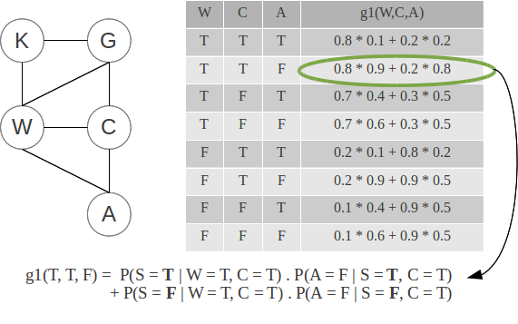
When eliminating S, we compute the inner-most sum: the first factor {$g1(W,C,A)$} is computed as a CPT (conditional probability table) over W, C and A:

We repeat this process for G, W and C: notice that CPT's for {$k$} binary variables store {$2^k$} values. We could very well directly compute {$P(K,G,W,C,S,A)$} as a big CPT and sum appropriate rows to obtain desired marginals, but variable elimination saves computations, and scales to much bigger networks (see example in the BN lecture).

Questions from past exams

Note that we covered somewhat different material this year than previous years, so some of the material below (e.g. "halving") will not be familiar to you and will not be on the final.

Shorts (2009 final)

• Suppose your friend told you that her SVM and logistic regression worked a lot better on her small dataset if she used feature selection first (she computed information gain of each feature and took the top 100 features). Why do you think generalization improved after feature selection?

(:ans:) Irrelevant features can hurt with small datasets. (:ansend:)

• You tell her that while most of the time feature selection can help, there are cases where it might throw away very good features... In particular, you tell her, this one time in CIS520, you were using a decision tree, and you did the same feature selection (taking top 100 features ranked by their information gain) and it really hurt your accuracy. Give a simple example where features might look uninformative in terms of information gain, but in fact be very useful.

(:ans:) {$y = x_1 \; {\rm XOR} \; x_2 $} (:ansend:)

• After hearing about the Netflix prize competition, you're convinced that the best classifier out there is a combination of many different classifiers. You build 100 different classifiers for the next competition, and then a friend tells you that she has another great one for you, but she wants a cut of the winnings. She won't give you the code, but she'll let you see the predictions of her classifier on a test set you give her. How would you decide whether her classifier might be useful in your ensemble?

(:ans:) If her classifier is accurate and make different errors than your current ensemble, start negotiating with her. (:ansend:)

EM this HMM (2008 final)

Consider a simple two-step HMM, with hidden states {$ (Z_1,Z_2) $} and observed variables {$ (O_1,O_2) $}. Let us denote the parameters of the HMM as:

{$ \; $\begin{align*} \theta_{Z_1=z_1} = & P(Z_1=z_1) \\ \theta_{Z_2=z_2|Z_1=z_1} = & P(Z_2=z_2|Z_1=z_1) \\ \theta_{O_i=o_i|Z_i =z_i}= & P(O_i=o_i | Z_i = z_i), \;\; i=1,2 \end{align*}$ \; $}

• Express the log-probability of a single example {$(z_1,z_2,o_1,o_2)$} in terms of {$\theta$}.

(:ans:) {$\log P(z_1,z_2,o_1,o_2) = \log(\theta_{Z_1=z_1}\theta_{O_1=o_1|Z_1=z_1}\theta_{Z_2=z_2|Z_1=z_1}\theta_{O_2=o_2|Z_2=z_2})$} (:ansend:)

• Express the log probability of {$m$} i.i.d. examples {$(z_1^j,z_2^j,o_1^j,o_2^j)$} in terms of {$\theta$}

(:ans:) {$\sum_{j=1}^m \log\theta_{Z_1=z_1^j}\theta_{O_1=o_1^j|Z_1=z_1^j}\theta_{Z_2=z_2^j|Z_1=z_1^j}\theta_{O_2=o_2^j|Z_2=z_2^j})$} (:ansend:)

• Write down the ML estimate (no need for the derivation) for {$\theta_{Z_2=z_2|Z_1=z_1}$} in terms of counts.

(:ans:) {$\theta_{Z_2=z_2|Z_1=z_1} = \frac{\sum_j \mathbf{1}(z_1^j=z_1,z_2^j=z_2)}{\sum_j \mathbf{1}(z_1^j=z_1)}$} (:ansend:)

• Write down the ML estimate (no need for the derivation) for {$\theta_{O_i=o_i|Z_i=z_i}$} in terms of counts.

(:ans:) {$\theta_{O_i=o_i|Z_i=z_i} = \frac{\sum_j \sum_i \mathbf{1}(z_i^j=z_i,o_i^j=o_i)}{\sum_j \sum_i \mathbf{1}(z_i^j=z_i)} $} (:ansend:)

• Now, we consider unlabeled examples (the {$Z_i$'s$} are missing), so we need to do EM. Write down {$Q(Z_1=z_1,Z_2=z_2|o_1^j,o_2^j)$} for the E-step in terms of parameters {$\theta$}.

(:ans:) {$Q(Z_1=z_1,Z_2=z_2|o_1^j,o_2^j) = \frac{\theta_{Z_1=z_1}\theta_{O_1=o_1^j|Z_1=z_1}\theta_{Z_2=z_2|Z_1=z_1}\theta_{O_2=o_2^j|Z_2=z_2}}{\sum_{z_1,z_2} \theta_{Z_1=z_1}\theta_{O_1=o_1^j|Z_1=z_1}\theta_{Z_2=z_2|Z_1=z_1}\theta_{O_2=o_2^j|Z_2=z_2}}$} (:ansend:)

• Write down the M-step update for {$\theta_{Z_2=z_2|Z_1=z_1}$} in terms of {$Q$}'s in the E-step.

(:ans:) {$\theta_{Z_2=z_2|Z_1=z_1} = \frac{\sum_j Q(Z_1=z_1,Z_2=z_2|o_1^j,o_2^j)}{\sum_j Q(Z_1=z_1|o_1^j,o_2^j)} \\ \\ (Q(Z_1=z_1|o_1^j,o_2^j) = \sum_{z_2} Q(Z_1=z_1,Z_2=z_2|o_1^j,o_2^j))$} (:ansend:)

• Write down the M-step update for {$\theta_{O_i=o_i|Z_i=z_i}$} in terms of {$Q$}'s in the E-step.

(:ans:) {$\theta_{O_i=o_i|Z_i=z_i} = \frac{\sum_j \sum_i Q(Z_i=z_i | o_1^j,o_2^j)\mathbf{1}(o_i^j=o_i)}{\sum_j \sum_i Q(Z_i=z_i | o_1^j, o_2^j)} $} (:ansend:)

Online Learning (2010 final)

In online learning, the halving algorithm is used to make predictions when there are {$N$} experts and it is assumed that one of the experts makes no mistakes. You've seen that the halving algorithm will make at most {$\log_2 N$} mistakes. However, if there are no perfect experts, then this algorithm will not work: since every expert might make mistakes, they will all eventually be eliminated. Instead of throwing away the experts that make mistakes, we can use the weighted majority algorithm and weight each expert by some {$0\leq \beta \leq 1$} if they make a mistakes. The algorithm is:

At each time step {$t = 1$} to {$T$}:

• Player observes the expert predictions {$h_{1,t},\dots,h_{N,t}$}, each having a weight {$w_{i,t}$} and predicts

{$\hat{y_t} = \arg\max_y \sum_i w_{i,t}{\bf 1}[h_{i,t}=y]$}

• Outcome {$y_t$} is revealed.
• Weights are updated using using the following formula:

{$ \; $ w_{i,t+1} = \begin{cases} \beta w_{i,t} & \text{if }h_{i,t}\not=y_t \\ w_{i,t} & \text{if }h_{i,t}=y_t \end{cases}$ \; $}

For the following questions, assume {$y \in \{0,1\}$}.

• For what value of {$\beta$} is this algorithm equivalent to the halving algorithm?

(:ans:) {$\beta = 0$} (:ansend:)

• Let {$W_t=\sum_i w_{i,t}$} be the sum of all weights at time {$t$}. If {$\beta = 1/3$}, show that when a mistake is made at time {$t$} then {$W_{t+1} \leq 2/3W_{t}$}.

(:ans:) If a mistake is made, then there must have been at least half the weight voting for it. The new weight is at most {$1/2 + (1/3)(1/2) = 3/6 + 1/6 = 4/6 = 2/3$}, giving {$W_{t+1} \leq 2/3W_{t}$}. (:ansend:)

• Suppose that there are {$N$} experts, each initialized with a weight of 1. Show that if {$M$} mistakes were made by time {$t$}, then {$W_{t} \leq N(2/3)^M$}.

(:ans:) The total weight at the beginning of the algorithm is {$n$}. Each time a mistake is made, the weight is reduced by at least 1/3. Since {$M$} mistakes were make, this happened {$M$} times, and so {$W_{t} \leq N(2/3)(2/3)\dots(2/3) = N(2/3)^M$}. (:ansend:)

• It turns out that this algorithm doesn't make many more mistakes than the best expert, which you will now show. If the best expert makes {$m$} mistakes, then its weight at time {$t$} will be {$(1/3)^m$}, and so the total weight will be at least that much: {$W_t \geq (1/3)^m$}. Combining this equation with your result from the previous question implies that {$(1/3)^m \leq N(2/3)^M$}. Use this inequality to show the following bound on the number of mistakes:

{$ M \leq \frac{1}{\log_3 3/2}[m+\log_3 N].$}

(:ans:) Starting with {$(1/3)^m \leq N(2/3)^M$}, we can take the log of both sides, giving {$ m\log_3(1/3) \leq \log_3 N + M\log_3(2/3).$}

Negating both sides gives {$m \geq -\log_3 N + M\log_3(3/2),$} and rearranging gives the desired result: {$M \leq \frac{1}{\log_3 3/2}\left[m+\log_3 N\right].$} (:ansend:)