BoostingDTs
Decision Trees and Cross-Validation
Suppose you are the owner of a pet store that sells bulldogs and goldfish. When a new customer comes into your store, you want to be able to recommend to them the pet that will make them happiest. Over the past few days you've recorded the answers of some satisfied customers to two questions you've posed:
- How many free hours do you have each week? (almost none, a few, many)
- How would you rate your fear of your neighbors? (high, low)
| {$X_1$} = Free hours per week | {$X_2$} = Fear of neighbors | {$Y$} = Pet type | Customer count |
|---|---|---|---|
| almost none | low | goldfish | 5 |
| almost none | low | bulldog | 5 |
| almost none | high | bulldog | 5 |
| a few | low | goldfish | 5 |
| a few | high | bulldog | 5 |
| many | low | goldfish | 5 |
| many | high | bulldog | 5 |
- Warm-up question: Using all the data in the above table as training data, what attribute will be split on first when using ID3 to create a decision tree?
Let {$n$}, {$f$}, and {$m$} stand for "almost none", "a few", and "many". Let {$g$} and {$b$} stand for "goldfish", and "bulldog". (:centereq:) {$ \; $ \begin{align*} H(Y \mid X_1) &= - \sum_{x \in \{n, f, m\}} P(X_1 = x) \sum_{y \in \{g, b\}} P(Y = y \mid X_1 = x) \log_2 P(Y = y \mid X_1 = x) \\ &= -1*\Bigg(\frac{15}{35}\Big(\frac{10}{15}\log_2\frac{10}{15} + \frac{5}{15}\log_2\frac{5}{15}\Big) + 2*\frac{10}{35}\Big(2*\frac{5}{10}\log_2\frac{5}{10}\Big)\Bigg) = 0.9650 \\ H(Y \mid X_2) &= -1*\Bigg(\frac{20}{35}\Big(\frac{15}{20}\log_2\frac{15}{20} + \frac{5}{20}\log_2\frac{5}{20}\Big) + \frac{15}{35}\Big(\frac{15}{15}\log_2\frac{15}{15}\Big)\Bigg) = 0.4636 \\ \end{align*} $ \; $} (:centereqend:)
ID3 will split on {$X_2$}, fear of neighbors, since it maximizes {$IG(X_i,Y) = H(Y) - H(Y \mid X_i)$}.
- Recall that cross-validation is a tool that can help determine optimal model complexity. Using leave-one-out cross-validation, determine whether it's better to ask your customers just one question, or to ask both questions. (Is cross-validation error lower with a decision tree of depth 1, or depth 2?) (:ans:)
Depth 1: No matter what point is left out, it is easy to see that the decision stump learned on the remaining data will be a split on {$X_2$}, fear of neighbors. Thus, over all leave-one-out cross-validation runs, the depth 1 trees will make mistakes only on the (almost none, low, bulldog) cases, for a total of {$5$} errors.
Depth 2: No matter what point is left out, depth 2 trees will always split on the fear of neighbors attribute first, just as the depth 1 trees do. In the "high" fear branch, no more splitting will occur because the level-1 leaf is pure. In the "low" fear branch however, a split on {$X_1$}, the free hours per week attribute, will occur. If the leave-one-out round is leaving out an (almost none, low, bulldog) point or an (almost none, low, goldfish) point, then this results in it's misclassification. The error total in the depth 2 case then comes to {$10$}.
Since cross-validation finds more errors in the depth 2 case than the depth 1, it's probably best to ask your customers just one question. The number of free hours they have each week seems irrelevant to whether they're happiest with a bulldog or a goldfish. (:ansend:)
Boosting
Some questions this example will answer:
- Will AdaBoost ever choose the same weak learner multiple times?
- How does the weighted training error {$\epsilon_t$} of the {$t$}-th classifier tend to change with respect to {$t$}?
- If allowed to run for an infinite amount of time, should AdaBoost always approach 0 training error?
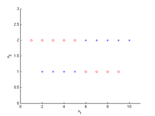
Suppose we want to use AdaBoost to learn a classifier for the data shown below. The output class is binary {$y \in \{1, -1\}$}, and the inputs are {$x_1, x_2 \in \mathbb{R}$}. Let the weak learners AdaBoost has access to be decision stumps; that is, any given weak learner's decision boundary is always parallel to one of the axes. In each iteration, assume the algorithm chooses the weak learner {$h_t(\mathbf{x})$} that maximizes classification accuracy with respect to the current weights: {$\sum_i D_t(i)\mathbf{1}(y^{(i)} \neq h_t(\mathbf{x}^{(i)})$}. Consider only decision boundaries that fall midway between data points (maximize margin).
- What is the first decision boundary AdaBoost will find?
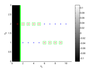
All points are equally weighted to begin with, so {$D_1(i) = 1/18$} for all {$i \in \{1 \ldots 18\}$}. Any split on {$x_2$} can at most get {$1/2$} the points correct. A split on {$x_1$} between any two points can do slightly better than this. Consider a decision boundary at {$x_1 = 1.5$}, such that {$x_1 < 1.5$} implies {$y = -1$} and {$x_1 > 1.5$} implies {$y = 1$}. This has error {$8/18 = 4/9$}.
- What is the second decision boundary AdaBoost will find?
Assuming the first classifier splits the data at {$x_1 = 1.5$}, consider the new data weights:
(:centereq:) {$ \; $ \begin{align*} \alpha_1 &= \frac{1}{2} \log\Bigg(\frac{1 - 8/18}{8/18}\Bigg) = 0.1116 \\ D_2((1,2)) &= \frac{D_1((1,2))\exp\{-\alpha_1 y_{(1,2)} h_1((1,2))\}}{Z_1} = \frac{\frac{1}{18} \exp\{-0.1116(-1)(-1)\}}{Z_1} = \frac{0.0497}{Z_1} \\ D_2((2,2)) &= \frac{D_1((2,2))\exp\{-\alpha_1 y_{(2,2)} h_1((2,2))\}}{Z_1} = \frac{\frac{1}{18} \exp\{-0.1116(-1)(1)\}}{Z_1} = \frac{0.0621}{Z_1} \\ D_2((2,1)) &= \frac{D_1((2,1))\exp\{-\alpha_1 y_{(2,1)} h_1((2,1))\}}{Z_1} = \frac{\frac{1}{18} \exp\{-0.1116(1)(1)\}}{Z_1} = \frac{0.0497}{Z_1} \\ Z_1 &= 10*0.0497 + 8*0.0621 = 0.9938 \\ \end{align*} $ \; $} (:centereqend:)
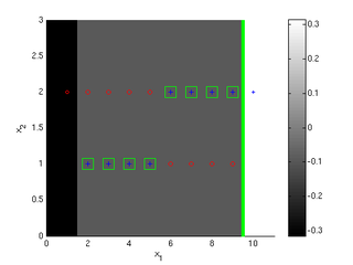
This shows the points the first classifier got wrong have higher weights in the second iteration. Now, if the second classifier places its decision boundary at {$x_2 = 1.5$} it will do slightly better than error {$1/2$}. However, it can get all the highly weighted negative examples correct if it places the decision boundary at {$x_1 = 9.5$}. So, this is the better choice. (Symmetrically, if the first classifier had instead been placed at {$x_1 = 9.5$}, the second classifier would be a split at {$x_1 = 1.5$}.)
- What is the third decision boundary AdaBoost will find?
At this point, both the 1st and 2nd classifiers correctly labeled the extreme left and right points (1,2) and (10,2). Each of the other points was misclassified by one of the first two classifiers and correctly classified by the other. Thus, we've reached a situation analogous to the one we started with: a split on {$x_2$} can at best achieve error {$1/2$}, and a split on {$x_1$} between any two points can do slightly better. So, as in part 1, we could choose the decision boundary to be at {$x_1 = 1.5$}.
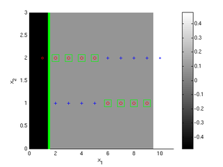
You can extend this reasoning to see that AdaBoost will in fact just flip-flop between these two decision boundaries, {$x_1 = 1.5$} and {$x_1 = 9.5$} for as long as it runs.
- Does the weighted training error of the {$t$}-th classifier increase or decrease as {$t \rightarrow \infty$}?
Initially, the error is {$8/18$}. Using the numbers we computed for {$D_2$} in part 2, we can compute {$\epsilon_2 = 0.4$}. So, initially it looks like the {$\epsilon_t$} decrease with {$t$}. However, flip-flopping between the two decision boundaries at {$x_1 = 1.5$} and {$x_1 = 9.5$}, the extreme points (1,2) and (10,2) will always be classified correctly and so their weights will approach 0 as {$t \rightarrow \infty$}, while the central points will slowly accrue all the mass. Thus, as {$t \rightarrow \infty$}, weighted training error of the {$t$}-th classifier increases: {$\epsilon_t \rightarrow 1/2$}.
(:centereq:) {$ \; $ \begin{align*} \epsilon_1 &= 8/18 = 0.4444 \\ \epsilon_2 &= 8*(0.0497/0.9938) = 0.4 \\ \epsilon_3 &= 0.4167 \\ \epsilon_4 &= 0.4286 \\ \epsilon_5 &= 0.4375 \\ \epsilon_6 &= 0.4444 \\ \epsilon_7 &= 0.4500 \\ \epsilon_8 &= 0.4545 \\ \epsilon_9 &= 0.4583 \\ \epsilon_{10} &= 0.4615 \\ \end{align*} $ \; $} (:centereqend:)
- Do the classifier confidences {$\alpha_t$} increase or decrease as {$t \rightarrow \infty$}? (:ans:)
As we saw in the previous part, the {$\epsilon_t$} increase with {$t$}. The {$\alpha_t$} are based entirely on the {$\epsilon_t$}:
(:centereq:) {$ \alpha_t = \frac{1}{2} \log\Bigg(\frac{1 - \epsilon_t}{\epsilon_t}\Bigg) $} (:centereqend:)
Thus, the {$\alpha_t$} decrease as {$t \rightarrow \infty$}. (:ansend:)
- What is the training error for the overall AdaBoost classifier {$y = h(\mathbf{x}) = sign(\alpha_1 h_1(\mathbf{x}) + \alpha_2h_2(\mathbf{x}) + \ldots)$} as {$t \rightarrow \infty$}?
Every other classifier will make the same 8 errors. So, overall error is {$\mathrm{error} = \frac{8}{18}$}.
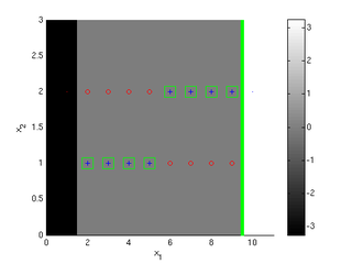
The plots below show the first 3 classifiers, and the 100th classifier. Darker shading indicates the overall AdaBoost classifier's value is more negative in a region, while lighter shading indicates it's more positive (colorbars give exact values). Points that are incorrectly classified by the overall classifier {$h = sign(\sum_t \alpha_t h_t)$} are shown with green boxes around them. The size of the points corresponds to their weight after the given iteration number; smaller size means smaller weight. Notice that by iteration 100 the extreme points have very little weight.
This example gives AdaBoost a bad rap. The problem here is that we've violated a fundamental assumption of boosting: we expect the weak classifiers we use to make a variety of different errors on the training data. That way, the different errors can cancel each other out. Unfortunately, in this problem choosing the best decision stumps results in weak classifiers that repeatedly make the same mistakes. This leads to {$\epsilon_t \rightarrow 1/2$} as {$t \rightarrow \infty$}, which means that the learning bound you will prove in the second homework
{$ \textrm{AdaBoost error} \leq \exp(-2\sum_t \gamma_t^2) $}
is useless; since {$\gamma = 1/2 - \epsilon_t = 0$} in the limit as {$t \rightarrow \infty$}, this bound just states error will be less than or equal to {$e^0 = 1$}. Thus, in this special case AdaBoost fails to learn anything useful.
Loss Functions: Boosting vs. Logistic Regression
From the class notes: Boosting vs. Logistic Regression
{$ \textrm{boosting error} = \frac{1}{n} \sum_i \mathbf{1}(f_\alpha(\mathbf{x}_i) \neq y_i) \leq \frac{1}{n} \sum_i \exp(-y_i f_\alpha(\mathbf{x}_i)) = \prod_t Z_t $}
If we choose each {$\alpha_t$} so that its value is: {$ \frac{1}{2} \log\Bigg(\frac{1 - \epsilon_t}{\epsilon_t}\Bigg) $}
then you can prove the resulting boosting algorithm (AdaBoost) is minimizing {$\prod_t Z_t = \prod_t \sum_i D_t(i) \exp(-\alpha_t y_i h_t(\mathbf{x}_i))$}, which is the same as minimizing {$\sum_i \exp(-y_i f_\alpha(\mathbf{x}_i))$}. This is an exponential loss function. In contrast, logistic regression maximizes a likelihood, which we can show is equivalent to minimizing the log loss function: {$\sum_i \log(1 + \exp(-y_i f_w(\mathbf{x}_i)))$}. The following derivation shows how maximizing logistic regression likelihood is identical to minimizing this log loss:
{$ \begin{align*} \arg\max_{\mathbf{w}}\;\; \textrm{likelihood} &= \arg\max_{\mathbf{w}}\;\; \prod_i P(y_i \mid \mathbf{x}_i, \mathbf{w}) \\ &= \arg\max_{\mathbf{w}}\;\; \prod_i \frac{1}{1 + \exp(-y_i \mathbf{w}^\top \mathbf{x}_i)} \\ &= \arg\max_{\mathbf{w}}\;\; \log\Bigg(\prod_i \frac{1}{1 + \exp(-y_i \mathbf{w}^\top \mathbf{x}_i)}\Bigg) \\ &= \arg\max_{\mathbf{w}}\;\; \sum_i (\log 1 - \log(1 + \exp(-y_i \mathbf{w}^\top \mathbf{x}_i))) \\ &= \arg\max_{\mathbf{w}}\;\; - \sum_i \log(1 + \exp(-y_i \mathbf{w}^\top \mathbf{x}_i)) \\ &= \arg\min_{\mathbf{w}}\;\; \sum_i \log(1 + \exp(-y_i \mathbf{w}^\top \mathbf{x}_i)) \\ \end{align*} $}
See the class notes for a discussion of the advantages of log versus exponential loss: Boosting vs. Logistic Regression.

