• View
• Edit
• History
• Print

SVMs

Support Vector Machines

Historically, Support Vector Machines (SVMs) were motivated by the notion of the maximum margin separating hyperplane. Before we explore this motivation, which is a bit of a MacGuffin, let's relate it to the other linear classification algorithms: we have seen that Logistic Regression and Boosting minimize a convex upper-bound on the $0/1$ loss for binary classification: logistic in one case and exponential in the other. Support Vector Machines minimize the hinge loss -- also an upper-bound on the $0/1$ loss.

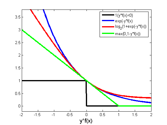
A few things to note about the hinge loss.

• It's convex like the exponential and logistic loss: optimization is fairly easy
• It grows slower below zero: the penalty for misclassification is more mild
• It is zero after 1: once correct and confident enough, there is no bonus for driving $y f(x)$ higher
• It's non-differentiable at the hinge point: simple gradient doesn't work

Why all the excitement about this loss? First, it has a nice geometric interpretation (at least in the linearly separable case) as leading to a maximum margin hyperplane separating positive from negative examples. Second, more importantly, it fits particularly well with kernels because many examples will not be a part of the solution, leading to a much more efficient dual representation and algorithms.

Hyperplanes and Margins

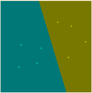
Consider the case of linearly separable data. In the toy 2D example below, there are many hyperplanes (lines) that separate the negative examples (blue) from positive (green). If we define the margin of a hyperplane as the distance of the closest point to the decision boundary, the maximum margin hyperplane is shown below.

We will denote our linear classifier as (note the constant term b is separated out)

$h(\mathbf{x}) = sign(\mathbf{w}^\top\mathbf{x} + b)$

Since rescaling the classifier by multiplying it by a positive constant does not change the decision boundary, $sign(\mathbf{w}^\top\mathbf{x} + b) = sign(\gamma (\mathbf{w}^\top\mathbf{x} + b))$, we will set the scale so that at the points closest to the boundary, $\mathbf{w}^\top\mathbf{x} + b = \pm 1$, as shown in the figure below.

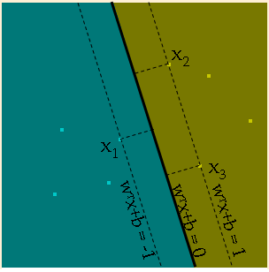
Now we will compute the margin, which is the distance of the points closest to the boundary, using one point from each class, $\mathbf{x}_1$ and $\mathbf{x}_2$.

$\mathbf{w}^\top\mathbf{x}_1 + b = -1 \; \; {\rm and} \;\; \mathbf{w}^\top\mathbf{x}_2 + b = 1$

Hence,

$\mathbf{w}^\top(\mathbf{x}_2-\mathbf{x}_1) = 2 \;\; \rightarrow \;\; \frac{\mathbf{w}^\top}{2||\mathbf{w}||_2}(\mathbf{x}_2-\mathbf{x}_1) = \frac{1}{||\mathbf{w}||_2}$

Note that $\frac{\mathbf{w}}{2||\mathbf{w}||_2}(\mathbf{x}_2-\mathbf{x}_1)$ is precisely the distance to the hyperplane: the vector $\frac{1}{2}(\mathbf{x}_2-\mathbf{x}_1)$ projected on the unit vector $\frac{\mathbf{w}}{||\mathbf{w}||_2}$. Let's restate this more precisely. A rescaled hyperplane classifier satisfies:

$y_i(\mathbf{w}^\top\mathbf{x}_i + b) \ge 1,\;\;\; i=1,\ldots,n$

(with equality for the closest points) and has margin $\frac{1}{||\mathbf{w}||_2}$.

To find the maximal margin hyperplane, we can simply maximize $\frac{1}{||\mathbf{w}||_2}$, which is equivalent to minimizing $\frac{1}{2}\mathbf{w}^\top\mathbf{w}$ subject to the (scaled) correct classification constraints. The SVM optimization problem (in the separable case) is:

$\; \begin{align*} & \textbf{Separable SVM primal:} \\ \min_{\mathbf{w},b}\;\; & \frac {1}{2}\mathbf{w}^\top\mathbf{w} \\ \textrm{s.t.}\;\; & y_i(\mathbf{w}^\top\mathbf{x}_i + b) \ge 1, \;\; i=1,\ldots,n \end{align*} \;$

Note on notation: I will use $\min/\max$ instead of $\inf/\sup$ since the continuous nature of the optimization will be obvious from context. This optimization problem has a quadratic objective and linear inequality constraints. Note that only the points closest to the boundary participate in defining the SVM hyperplane. These points are called the support vectors, and we will see that the solution can be expressed only using these points.

The Dual View

In order to get more intuition about the problem, we can look at it from the dual perspective. Lagrangian duality provides the right tool here. We formulate the Lagrangian by introducing a non-negative multiplier $\alpha_i$ (the Lagrange multiplier, which we called $\lambda$ before) for each inequality constraint:

$L(\mathbf{w},b,\alpha) = \frac{1}{2}\mathbf{w}^\top\mathbf{w} + \sum_i \alpha_i (1-y_i(\mathbf{w}^\top\mathbf{x}_i + b))$

Note that if $\mathbf{w},b$ is feasible (i.e. satisfy all the constraints), then:

$\; \begin{equation*} \max_{\alpha\ge 0} L(\mathbf{w},b,\alpha) = \frac{1}{2}\mathbf{w}^\top\mathbf{w} \end{equation*} \;$

since all the coefficients $(1-y_i(\mathbf{w}^\top\mathbf{x}_i + b))$ are negative or zero. When $\mathbf{w},b$ are not feasible, $\max_{\alpha\ge 0} L(\mathbf{w},b,\alpha)= \infty$. Assuming that feasible $\mathbf{w},b$ exist, $\min_{\mathbf{w},b} (\max_{\alpha\ge 0} L(\mathbf{w},b,\alpha))$ solves the original problem, and since the original objective is convex (and assuming it's feasible for a moment), we can change the order of $\min/\max$ to obtain a dual problem that has the same optimal value: $\max_{\alpha\ge 0} (\min_{\mathbf{w},b} L(\mathbf{w},b,\alpha))$. Taking derivatives with respect to $\mathbf{w}$ and b and setting them to zero, we get:

$\frac{\partial L}{\partial b} = 0 \;\; \rightarrow \;\; \sum_i \alpha_i y_i = 0$

and

$\frac{\partial L}{\partial \mathbf{w}} = 0 \;\; \rightarrow \;\; \mathbf{w} = \sum_i \alpha_i y_i \mathbf{x}_i$

Note the dual representation of $\mathbf{w}$: it is a linear combination of the examples, weighted by dual variables $\alpha_i$. Plugging in the expression for $\mathbf{w}$, we get:

$\; \begin{align*} L(b,\alpha) & = \frac{1}{2}\sum_{i,j} \alpha_i\alpha_j y_i y_j\mathbf{x}_i^\top\mathbf{x}_j+ \sum_i \alpha_i (1-y_i(\sum_j \alpha_j y_j\mathbf{x}_j^\top\mathbf{x}_i + b)) \\ & = - \frac{1}{2}\sum_{i,j} \alpha_i\alpha_j y_i y_j\mathbf{x}_j^\top\mathbf{x}_i+ \sum_i \alpha_i - \sum_i \alpha_i y_i b \end{align*} \;$

Since $\sum_i \alpha_i y_i = 0$, the dual problem is:

$\; \begin{align*} & \textbf{Separable SVM dual:} \\ \max_{\alpha\ge 0}\;\; & \sum_i \alpha_i - \frac{1}{2}\sum_{i,j} \alpha_i\alpha_j y_i y_j\mathbf{x}_i^\top\mathbf{x}_j \\ \textrm{s.t.}\;\; & \sum_i \alpha_i y_i = 0 \end{align*} \;$

This dual optimization problem, as the primal, has a quadratic objective and (a single) linear constraint. Because of the (KKT) optimality conditions, when $\mathbf{x}_i$ is not the closest to the boundary, $\alpha_i$ is zero. So only the points that support the hyperplane, called support vectors, participate in the solution. Given a solution $\alpha$ to the problem, we can recover the primal via: $\mathbf{w} = \sum_i \alpha_i y_i \mathbf{x}_i$ To recover $b$, note that for any support vector $i$, where $\alpha_i>0$, we have $y_i(\mathbf{w}^\top\mathbf{x}_i+b)=1$, so

$b = y_i-\mathbf{w}^\top\mathbf{x}_i, \;\; \forall i\;\; \alpha_i > 0.$

Kernels

We can use the kernel trick again, by assuming a feature map $\phi(\mathbf{x})$ such that $k(\mathbf{x}_i,\mathbf{x}_j) = \phi(\mathbf{x}_i)^\top\phi(\mathbf{x}_j)$. The kernelized dual optimization problem is:

$\; \begin{align*} & \textbf{Kernelized separable dual:} \\ \max_{\alpha\ge 0}\;\; & \sum_i \alpha_i - \frac{1}{2}\sum_{i,j} \alpha_i\alpha_j y_i y_jk(\mathbf{x}_i,\mathbf{x}_j) \\ \textrm{s.t.}\;\; & \sum_i \alpha_i y_i = 0 \end{align*} \;$

Given a solution $\alpha$ to the problem, we can recover

$b = y_i-\sum_j\alpha_j y_j k(\mathbf{x}_j,\mathbf{x}_i)\;\; \forall i\;\; \alpha_i > 0$

and the prediction:

$\mathbf{w}^\top \mathbf{x} +b = \sum_i \alpha_i y_i k(\mathbf{x}_i,\mathbf{x}) + b$

Non-separable case

When the data is not separable, the above optimization will fail. Consider the case in the figure below, where the yellow point in the center of the blue ones cannot be separated from the blue and grouped with the other yellow using any linear separator.

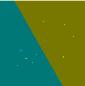
In general, if data is non-separable this means that for at least one data point, say the $r$th point, the $y_r(\mathbf{w}^\top\mathbf{x}_r + b)$ term will fail to exceed the threshold value 1 no matter what $\mathbf{w}$ is set to. This will mean the $\max_{\alpha} L(\mathbf{w},b,\alpha)$ optimization can achieve value $\infty$ by setting $\alpha_r = \infty$. The resulting classifier $h(\mathbf{x}) = sign(\alpha_r y_r \mathbf{x}_r^\top \mathbf{x})$ will then depend only on comparison to the $r$th point. In practice, this means we'll be classifying all new data based on an outlier from the training set. This will likely give catastrophically low accuracy.

Although we might perhaps like to minimize the number of misclassified points, this is an NP-hard problem. Instead, to handle the case of points on the wrong side of the fence, SVMs introduce slack variables. These variables allow all the constraints to be satisfied, so that no $\alpha_i$ get set to $\infty$. A corresponding slack variable penalty term is added to the objective, such that the more the slack variables are relied upon, the worse the value of the objective.

Specifically, SVMs add a slack variable $\xi_i$ for each example so that the margin constraints become: $y_i(\mathbf{w}^\top\mathbf{x}_i + b) \ge 1 - \xi_i$. For $\xi_i > 0$ this means we allow points to be within the margin (or even on the wrong side of the linear separator for large enough $\xi_i$). The $\xi_i$ are then added as a penalty term in the objective, weighted by the positive slack penalty constant $C$:

$\; \begin{align*} & \textbf{Hinge primal:} \\ \min_{\mathbf{w},b,\xi\ge0}\;\; & \frac {1}{2}\mathbf{w}^\top\mathbf{w} + C\sum_i\xi_i \\ \textrm{s.t.}\;\; & y_i(\mathbf{w}^\top\mathbf{x}_i + b) \ge 1-\xi_i, \;\;\ i=1,\ldots,n \end{align*} \;$

The reason we call the primal for the non-separable case the hinge primal is that the value of $\xi_i$ can be written:

$\xi_i = \max(0,1-y_i(\mathbf{w}^\top \mathbf{x}_i +b))$

which is exactly the form of hinge loss (see the figure at the top of these lecture notes for a reminder of what the hinge function looks like). That is, using these $\xi_i$ we are penalizing linearly for misclassification.

Taking the dual, we get:

$\; \begin{align*} & \textbf{Hinge dual:} \\ \max_{\alpha\ge 0}\;\; & \sum_i \alpha_i - \frac{1}{2}\sum_{i,j} \alpha_i\alpha_j y_i y_j\mathbf{x}_i^\top\mathbf{x}_j \\ \textrm{s.t.}\;\; & \sum_i \alpha_i y_i = 0,\;\; \alpha_i\le C,\;\; i=1,\ldots,n \end{align*} \;$

Notice that this is exactly the same as the separable dual, but with the added constraints $\alpha_i\le C$. So, adding the slack variables $\xi_i$ in the primal amounts to putting a cap on $\alpha_i$ in the dual. Effectively, the cap limits the extent to which any one point can influence the final classifier, $h(\mathbf{x}) = sign(\sum_i \alpha_i y_i \mathbf{x}_i^\top\mathbf{x})$.

Here's a short derivation of the dual. In addition to the $\alpha$s, we introduce a non-negative Lagrange multiplier $\lambda_i$ for each $\xi_i \ge 0$ constraint.

$\; \begin{align*} L(\mathbf{w},b,\xi,\alpha,\lambda) & = \frac{1}{2}\mathbf{w}^\top\mathbf{w} + C\sum_i \xi_i + \sum_i \alpha_i (1-\xi_i-y_i(\mathbf{w}^\top\mathbf{x}_i + b)) - \sum_i \lambda_i \xi_i \\ \frac{\partial L}{\partial b} & = 0 \;\; \rightarrow \;\; \sum_i \alpha_i y_i = 0 \\ \frac{\partial L}{\partial \mathbf{w}} & = 0 \;\; \rightarrow \;\; \mathbf{w} = \sum_i \alpha_i y_i \mathbf{x}_i \\ \frac{\partial L}{\partial \xi_i} & = 0 \;\; \rightarrow \;\; C -\alpha_i - \lambda_i= 0 \end{align*} \;$

Plugging in the expression for $\mathbf{w}$ and using the condition $\sum_i \alpha_i y_i = 0$ as before, we have

$L(\xi,\alpha,\lambda) = \sum_i \alpha_i - \frac{1}{2}\sum_{i,j} \alpha_i\alpha_j y_i y_j\mathbf{x}_i^\top\mathbf{x}_j + \sum_i \xi_i (C-\alpha_i - \lambda_i)$

Now using the condition $C -\alpha_i - \lambda_i= 0$, the last sum vanishes, so we are left with the dual:

$\; \begin{align*} \max_{\alpha\ge 0,\lambda\ge 0}\;\; & \sum_i \alpha_i - \frac{1}{2}\sum_{i,j} \alpha_i\alpha_j y_i y_j\mathbf{x}_i^\top\mathbf{x}_j \\ \textrm{s.t.}\;\; & \sum_i \alpha_i y_i = 0, \;\;\ C-\alpha_i - \lambda_i=0 \end{align*} \;$

We can get rid of $\lambda_i$s by noting that they only appear in the constraint $C-\alpha_i - \lambda_i=0$, and since they must be non-negative, we can just replace the constraint with $C \ge \alpha_i$, as in the dual stated above. That is, the original constraint tells us $C - \alpha_i = \lambda_i$ and the only restriction on $\lambda_i$ is that it must be non-negative, so it's entire functionality can be captured by swapping in the constraint that $C - \alpha_i$ must be non-negative.

The kernelized version of the dual, analogous to the separable SVM case, is just:

$\; \begin{align*} & \textbf{Hinge kernelized dual:} \\ \max_{\alpha\ge 0}\;\; & \sum_i \alpha_i - \frac{1}{2}\sum_{i,j} \alpha_i\alpha_j y_i y_jk(\mathbf{x}_i,\mathbf{x}_j) \\ \textrm{s.t.}\;\; & \sum_i \alpha_i y_i = 0,\;\; \alpha_i\le C,\;\; i=1,\ldots,n\end{align*} \;$

where $k(\mathbf{x}_i, \mathbf{x}_j)$ is substituted for $\mathbf{x}_i^\top\mathbf{x}_j$.

Given a solution $\alpha$ to the problem, we can recover

$b = y_i-\sum_j\alpha_j y_j k(\mathbf{x}_j,\mathbf{x}_i)\;\; \forall i\;\; C > \alpha_i > 0$

and the prediction:

$\mathbf{w}^\top \phi(\mathbf{x}) +b = \sum_i \alpha_i y_i k(\mathbf{x}_i,\mathbf{x}) + b$

Solving SVMs

We will not spend too much time on how to optimize quadratic programs with linear constraints. There is a very large literature on the topic of general convex optimization and SVM optimization in particular, and many off-the-shelf efficient tools have been developed for both. In recent years, simple algorithms (e.g., SMO, subgradient) that find approximate answers to the SVM problem have been shown to work quite well. Here is a an applet for kernel SVMs in 2D.

SVM Notation for different Objective Functions

As seen above, we have expressed the hinge primal as:

$\; \begin{align*} & \textbf{Hinge primal:} \\ \min_{\mathbf{w},b,\xi\ge0}\;\; & \frac {1}{2}\mathbf{w}^\top\mathbf{w} + C\sum_i\xi_i \\ \textrm{s.t.}\;\; & y_i(\mathbf{w}^\top\mathbf{x}_i + b) \ge 1-\xi_i, \;\;\ i=1,\ldots,n \end{align*} \;$

To generalize this slightly, we can write:

$\; \begin{align*} & \textbf{Hinge primal:} \\ \min_{\mathbf{w},b,\xi\ge0}\;\; & \frac {1}{2}\|\mathbf{w}\|_p^p + C\|\mathbf{\xi}\|_q^q \\ \textrm{s.t.}\;\; & y_i(\mathbf{w}^\top\mathbf{x}_i + b) \ge 1-\xi_i, \;\;\ i=1,\ldots,n \end{align*} \;$

Here, $\|\mathbf{w}\|_p^p$ is the p-norm of $\mathbf{w}$ raised to the p'th power, and likewise for $\|\mathbf{\xi}\|_q^q$. We often describe this as the objective for Lp-regularized, Lq-loss SVM. We can think of the $\mathbf{w}$ term is the regularization term (penalizes large model weights) and the $\|\mathbf{\xi}\|$ term as the loss term (penalizes large losses). The original hinge primal we derived is therefore L2-regularized, L1-loss SVM.

Back to Lectures