EM
Mixtures of Gaussians and Expectation Maximization
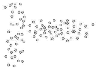
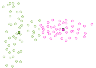
The K-means algorithm turns out to be a special case of clustering with a mixture of Gaussians where all variances are equal (and covariances are 0 and mixture weights are equal, as we'll see below): the underlying assumption is that clusters are essentially spherical. This assumption is clearly suboptimal for many situations. Here's an example where the clusters are not spherical and K-means cannot separate them:
More generally, different clusters may be on different scales, or may overlap, etc . Here's a nice applet that illustrates Mixtures of Gaussians.
Gaussian Mixtures
A probabilistic approach to clustering is to assume that the data is generated from a set of K simple distributions, in our current case, Gaussians:
{$p(\mathbf{x}) = \sum_{k=1}^K \pi_k N(\mu_k,\Sigma_k)$}
where {$\pi_k$} is the probability that a sample is drawn from {$k$}th mixture component. Note that {$\sum_{k=1}^K \pi_k = 1$} and {$\pi_k > 0$}. Another way to think about this model is to introduce a hidden variable {$z \in \{1,\ldots,K\}$} for each sample {$i$}, which indicates what mixture component it came from.
{$p(\mathbf{x}) = \sum_{k=1}^K p(z=k) p(\mathbf{x}\mid z=k)$}
where {$p(z=k) = \pi_k$} and {$p(\mathbf{x}\mid z=k) = N(\mu_k,\Sigma_k)$}.
Given a sample {$D=\mathbf{x}_1,\ldots,\mathbf{x}_n$}, the goal is to estimate the parameters of the mixture {$(\pi_k,\mu_k,\Sigma_k)$} for {$k=1,\ldots,K$}. As usual, we estimate the parameters using MLE (or MAP):
{$\log P(D \mid \pi,\mu,\Sigma) = \sum_i \log \sum_k p_\pi(z_i=k) p_{\mu,\Sigma}(\mathbf{x}_i\mid z_i=k)$}
Variance parameters
There are several common choices in learning variances of Gaussian mixtures.
- Full covariance: {$\Sigma_k$} is arbitrary for each class (clusters are general ellipsoids, {$O(Km^2/2)$} parameters)
- Shared Full covariance: {$\Sigma_k$} is arbitrary but same for each class (all clusters have same ellipsoid shape, {$O(m^2 / 2)$} parameters)
- Diagonal (aka Naive Bayes): {$\Sigma_k$} is a diagonal matrix (clusters are axis-aligned ellipsoids, {$O(Km)$} parameters)
- Shared Diagonal: {$\Sigma_k$} is a diagonal matrix but same for each class (all clusters have same axis-aligned ellipsoid shape, {$O(m)$} parameters)
- Spherical: {$\Sigma_k$} is {$\sigma_k I$} (clusters have spherical shape)
- Shared Spherical: {$\Sigma_k$} is {$\sigma I$} (all clusters have same radius)
Perhaps the most common is diagonal, especially when the number of dimensions is large.
Mixture parameters
There are two choices in learning mixture weights {$\pi_k$}.
- Equal weights: {$\pi_k = 1/K$}
- Arbitrary weights
K-Means
K-means can be seen as trying to find the values of hidden variables {$z_i$} (cluster assignments) and fit the mixture model assuming mixture weights are equal, {$\pi_k = 1/K$}, and variances are shared spherical, {$\Sigma_k = \sigma I$}, (the value of {$\sigma$} doesn't change the optimal {$\mathbf{z}$} and {$\mu$}, so we can just assume it's fixed).
{$\arg \max_{\mathbf{z},\mu} \log P(D, \mathbf{z} \mid \pi, \mu, \sigma) = \arg\max_{\mathbf{z},\mu} \sum_i \log (p_{\pi}(z_i)p_{\mu,\sigma}(\mathbf{x}_i | z_i)) = $} {$\arg\max_{\mathbf{z},\mu} \sum_i (\log 1/K + \log N(\mathbf{x}_i; \mu_{z_i},\sigma )) = $} {$\arg\min_{\mathbf{z},\mu} \sum_i \frac{||\mu_{z_i}-\mathbf{x}_i||^2}{2\sigma^2} = \arg\min_{\mathbf{z},\mu} \sum_i ||\mu_{z_i}-\mathbf{x}_i||^2$}
Note that this could alternatively be written as {$ \arg\min_{\mathbf{z},\mu} \sum_i \sum_{k} r_{ik}||\mu_{k}-\mathbf{x}_i||^2$} where {$ r_{ik}$} is an indicator function specifying which cluster {$x_i$} is in; this is the "hard clustering limit" of the GMM.
Expectation maximization
EM is a very general algorithm for learning models with hidden variables. EM optimizes the marginal likelihood of the data (likelihood with hidden variables summed out). Like K-means, it's iterative, alternating two steps, E and M, which correspond to estimating hidden variables given the model and then estimating the model given the hidden variable estimates. Unlike K-means, the cluster assignments in EM for Gaussian mixtures are soft. Let's consider the simplest case, closest to K-means.
EM for Gaussian mixtures with {$\Sigma_k = \sigma I$} ({$\sigma$} fixed a priori) and {$\pi_k = 1/K$}
- Init: randomly choose {$\mu_1$},.., {$\mu_K$}
- Alternate until convergence:
- E: Estimate {$P(z_i = k \mid \mathbf{x}_i) \propto \exp \{- ||\mu_{k}-\mathbf{x}_i||^2/2\sigma^2\} $}
- M: Estimate new {$\mu_k$}: {$\mu_k = \frac{\sum_i P(z_i = k \mid \mathbf{x}_i) \mathbf{x}_i}{\sum_i P(z_i = k \mid \mathbf{x}_i)}$}
The only difference from K-means is that the assignments to cluster are soft (probabilistic).
Now if we allow {$\Sigma$} and {$\pi$} to be arbitrary, we have:
EM for Gaussian mixtures
- Init: randomly choose {$\pi,\mu,\Sigma$}
- Alternate until convergence:
- E: Estimate {$P(z_i = k \mid \mathbf{x}_i) \propto \pi_k N(\mathbf{x}_i ; \mu_k,\Sigma_k)$}
- M: Estimate new {$\mu_k$}: {$\mu_k = \frac{\sum_i P(z_i = k \mid \mathbf{x}_i) \mathbf{x}_i}{\sum_i P(z_i = k \mid \mathbf{x}_i)}$}, {$\pi_k = \frac{1}{n}\sum_i P(z_i = k \mid \mathbf{x}_i)$} and {$\Sigma_k = \frac{\sum_i P(z_i = k \mid \mathbf{x}_i) (\mathbf{x}_i-\mu_k)(\mathbf{x}_i-\mu_k)^\top}{\sum_i P(z_i = k \mid \mathbf{x}_i)}$}
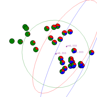
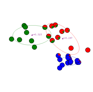
Example from Andrew Moore's tutorial:
EM in general
Recall that we are trying to find the MLE over a model with e.g. parameters {$\theta = (\pi,\mu,\Sigma)$} for observed data {$D = {\bf X}$}.
I.e., we want to find the {$\arg \max$} over {$\theta$} of
{$\log P(D \mid \theta) = \sum_i \log \sum_z p_\theta(Z_i=z,\mathbf{x}_i) = \sum_i \log \sum_k p_\pi(z_i=k) p_{\mu,\Sigma}(\mathbf{x}_i|z_i=k)$}
Why not just use gradient ascent?
Let's look in more detail at how the EM algorithm works. We will see that it is a sort of gradient ascent in likelihood, alternating between estimating how much each point belongs to each cluster, and estimating the parameters in the PDF that for each cluster that generates the observed points.
The E-step assumes we have estimates of the parameters {$\theta_j^{t-1}$} in the probability distribution for each cluster {$j$}, and then estimates the probability of each observed point {$\mathbf{x}_i$} being generated by each cluster : {$p(z_j|\mathbf{x}_i,\theta^{t-1})$}. This can be thought of as a "degree of membership" in the cluster.
The M-step assumes we know this probability of each observed point being generated by each cluster, and estimates the parameters {$\theta_j^{t}$} in the probability distribution for each cluster, computing an MLE in which each point's contribution to each cluster is weighted by the probability the point came from that cluster.
EM as optimization
EM is optimizing marginal likelihood, albeit in somewhat indirect way (say as opposed to simple gradient).
{$\log P(D \mid \theta) = \sum_i \log \sum_z p_\theta(Z_i=z,\mathbf{x}_i)$}
In order to analyze what EM is doing, we will define, for each example i, a distribution over the hidden variable {$q(Z_i \mid \mathbf{x}_i)$}. Then, we'll multiply and divide by this term:
{$\log P(D \mid \theta) = \sum_i \log \sum_z q(Z_i=z \mid \mathbf{x}_i) \frac{p_\theta(Z_i=z,\mathbf{x}_i)}{q(Z_i=z\mid\mathbf{x}_i)}.$}
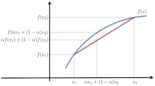
For scalar concave functions {$f(v)$} (such as {$\log$}), for all {$ (v_1, v_2), \alpha$} such that {$0 \leq \alpha \leq 1$}:
{$\alpha f(v_1) + (1 - \alpha) f(v_2) \leq f(\alpha v_1 + (1 - \alpha)v_2).$}
In words, interpolation underestimates concave functions.
More generally, given K values {$(v_1, \ldots, v_K)$} and K non-negative {$\alpha$} values {$(\alpha_1, \ldots, \alpha_K)$} such that
{$\sum _{k=1}^K\alpha_k = 1$},
we have Jensen's inequality,
{$\sum_{k=1}^K \alpha_k f(v_k) \leq f(\sum_{k=1}^K \alpha_k v_k).$}
In our setting, for each example i, the role of {$\alpha_k$} is played by {$q(Z_i=z|x_i)$} and the role of {$v_k$} is played by
{$\frac{p_\theta(Z_i=k,\mathbf{x}_i)}{q(Z_i=k\mid\mathbf{x}_i)}.$}
which we can use to get a lower-bound on our objective:
{$\log P(D \mid \theta) \ge \sum_i \sum_z q(Z_i=z \mid \mathbf{x}_i) \log \frac{p_\theta(Z_i=z,\mathbf{x}_i)}{q(Z_i=z\mid\mathbf{x}_i)} = F(q,\theta)$}
We have an objective function {$F(q, \theta)$}, which we can maximize in order to maximize {$\log P(D \mid \theta)$}. We can also show that local maxima of F are local maxima of {$\log P(D \mid \theta)$}, so we can just worry about maximizing F (see Neal and Hinton paper). The E and M step of EM are coordinate ascent steps on q and {$\theta$}, respectively.
{$F(q,\theta) = \sum_i \sum_z q(Z_i=z \mid \mathbf{x}_i) \log \frac{p_\theta(Z_i=z \mid \mathbf{x}_i)p_{\theta}(\mathbf{x}_i)}{q(Z_i=z\mid\mathbf{x}_i)} = \sum_i \left( -KL(q(Z_i \mid \mathbf{x}_i) \parallel p_\theta(Z_i \mid \mathbf{x}_i)) + \log p_\theta(\mathbf{x}_i)\right)$}
Hence maximizing {$F$} over q in the E-step leads to {$q(Z_i=z \mid \mathbf{x}_i) = p_\theta(Z_i=z \mid \mathbf{x}_i)$}, since {$p_\theta(\mathbf{x}_i)$} does not depend on {$q$}.
Also
{$F(q,\theta) = \sum_i \sum_z q(Z_i=z \mid \mathbf{x}_i) \log \frac{p_\theta(Z_i=z,\mathbf{x}_i)}{q(Z_i=z\mid\mathbf{x}_i)} = \sum_i \left( H(q(Z_i \mid \mathbf{x}_i)) + \sum_z q(Z_i=z \mid \mathbf{x}_i) \log p_\theta(Z_i=z,\mathbf{x}_i)\right)$}
Above, {$H(q(Z_i \mid \mathbf{x}_i))$} is the entropy, which doesn't depend on {$\theta$}. Hence maximizing F over {$\theta$} in the M-step is equivalent to an MLE where labeled examples {$(z, \mathbf{x}_i )$} are weighted by {$q(Z_i = z \mid \mathbf{x}_i)$}. The overall algorithm is:
General EM Algorithm
- Input: Model: {$p(z,\mathbf{x} \mid \theta)$}, starting parameters {$\theta^0$}, unlabeled data {$\mathbf{x}_1,\ldots,\mathbf{x}_n$}.
- For {$t=1, \ldots, T$} (until convergence criterion is met)
- E-step: {$q^t(Z_i|\mathbf{x}_i) = \arg\max_q F(q,\theta^{t-1}) = p(Z_i|\mathbf{x}_i,\theta^{t-1})$}
- M-step: {$\theta^t = \arg\max_\theta F(q^t,\theta) = \arg\max_\theta \sum_i \sum_z q^t(Z_i=z|\mathbf{x}_i)\log p_\theta(z,\mathbf{x}_i)$}
The beauty of this algorithm is that it decomposes nicely into two simple steps: computing the posterior over hidden variables using current parameters (E-step) and then using these posteriors to do (weighted) MLE on labeled data. EM is used not just for fitting mixture models, but also much more complicated models we'll talk about later, like Hidden Markov Models.
EM for mixtures with fixed shared diagonal variance
Let's derive the EM algorithm for fixed shared diagonal variance case {$\Sigma_k = \sigma I$}. The generative model has parameters {$(\pi_k,\mu_k)$} for each cluster where {$\mu_k$} is of dimension m. {$P(\mathbf{x}) = \sum_{k=1}^K \pi_k N(\mathbf{x}; \mu_k,\sigma I)$} We have our lower-bound function: {$ F(q,\pi,\mu) = const + \sum_i \sum_k q(Z_i=k|\mathbf{x}_i) \log (\pi_k e^{-||\mathbf{x_i}-\mu_k||^2/2\sigma^2}) $} The constant above comes from the constant of the Gaussian distribution.
For the E-step we have for each example:
- E-step:
{$ q^t(Z_i=k|\mathbf{x}_i) \propto p(Z_i=k,\mathbf{x}_i\mid\pi_k^{t-1},\mu_k^{t-1}) \propto \pi_k^{t-1} e^{-||\mathbf{x_i}-\mu_k^{t-1}||^2/2\sigma^2} $} The normalization constant for each example is determined by making sure q sums to 1 over k.
- M-step for {$\mu_k$}: collecting terms that depend on {$\mu_k$}, we have:
{$ \frac{\partial F(q^t,\pi,\mu)}{\partial \mu_k} = \sum_i q(Z_i=k|\mathbf{x}_i) (\mathbf{x_i}-\mu_k)/\sigma^2 $} Setting the derivative to zero and solving for {$\mu_k$}, we get: {$\mu_k = \frac{\sum_i q(Z_i = k \mid \mathbf{x}_i) \mathbf{x}_i}{\sum_i q(Z_i = k \mid \mathbf{x}_i)}$}
- M-step for {$\pi_k$}: Since {$ \sum_{k=1}^K \pi_k = 1$}, we need to add the constraint to the optimization (only terms that depend on {$\pi$} are kept):
{$\max_\pi \sum_i \sum_k q^t(Z_i=k|\mathbf{x}_i)\log \pi_k \;\; {\rm s.t.}\;\; \sum_{k=1}^K \pi_k = 1. $} We form the Lagrangian: {$L(\pi, \lambda) = \sum_i \sum_k q^t(Z_i=k|\mathbf{x}_i)\log \pi_k - \lambda (\sum_{k=1}^K \pi_k - 1)$} and take the derivative with respect to {$\pi$}: {$ \frac{\partial L(\pi,\lambda)}{\partial \pi_k} = \sum_i \frac{q^t(Z_i=k|\mathbf{x}_i)}{\pi_k} - \lambda $} Setting the derivative to zero gives us: {$\pi_k = \frac{1}{\lambda}\sum_i q^t(Z_i=k|\mathbf{x}_i) $} Now, we can just guess that {$\lambda = n$}, but let's do this more formally, by plugging the expression for {$\pi_k$} back into the Lagrangian, but for convenience, let's define {$c_k = \sum_i q^t(Z_i=k|\mathbf{x}_i)$}, then we have
{$\min_\lambda \; \sum_i \sum_k q^t(Z_i=k|\mathbf{x}_i)(\log c_k - \log \lambda) - (\sum_k c_k ) + \lambda $}
Now we eliminate terms that don't depend on {$\lambda$} and noting that {$\sum_i \sum_k q^t(Z_i=k|\mathbf{x}_i) = n$} to get the dual: {$\min_\lambda \; - n \log \lambda + \lambda $} Setting the derivative to 0 gives us {$\lambda = n$}.
More references
- EM math for a GMM: a clean walk-through of the EM math for a GMM; (the code in R, but reasonably comprehensible)
- numpy code: less clear math, but has numpy code and pointers to other references

