DecisionTrees
Decision Trees
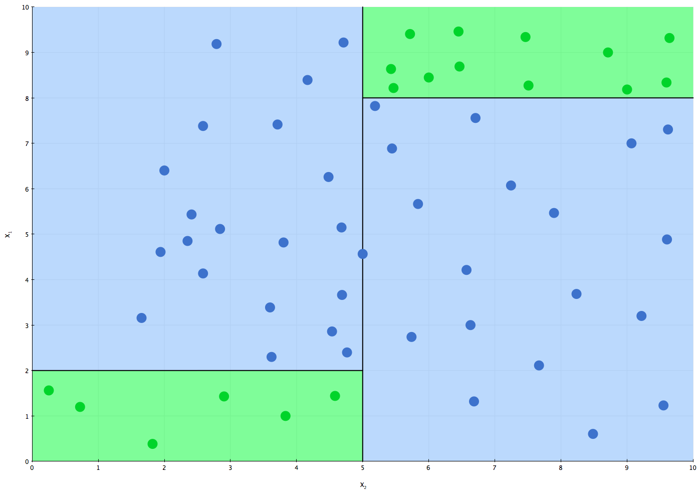
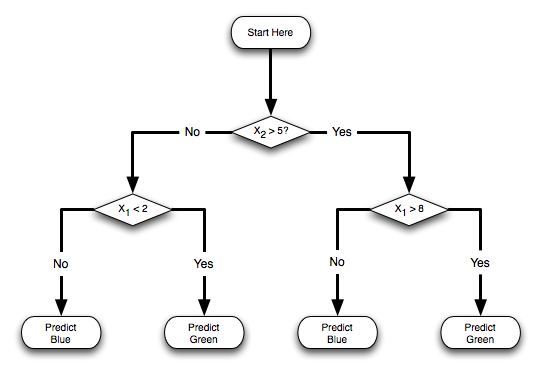
After the Nearest Neighbor approach to classification/regression, perhaps the second most intuitive model is Decision Trees. Below is an example of a two-level decision tree for classification of 2D data. Given an input x, the classifier works by starting at the root and following the branch based on the condition satisfied by x until a leaf is reached, which specifies the prediction.
 |  |
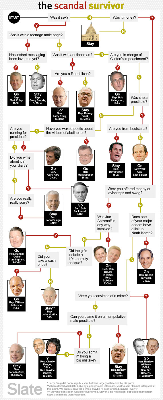
Here's a more complicated example courtesy of The Slate:
 |
Here are decision trees (forests, actually) in action!!

An example with data
Consider trying to predict Miles per Gallon (MPG) for a set of cars using the following dataset.
| mpg | cylinders | displacement | horsepower | weight | acceleration | modelyear | maker |
|---|---|---|---|---|---|---|---|
| Bad | 8 | 350 | 150 | 4699 | 14.5 | 74 | America |
| Bad | 8 | 400 | 170 | 4746 | 12 | 71 | America |
| Bad | 8 | 400 | 175 | 4385 | 12 | 72 | America |
| Bad | 6 | 250 | 72 | 3158 | 19.5 | 75 | America |
| Bad | 8 | 304 | 150 | 3892 | 12.5 | 72 | America |
| Bad | 8 | 350 | 145 | 4440 | 14 | 75 | America |
| Bad | 6 | 250 | 105 | 3897 | 18.5 | 75 | America |
| Bad | 6 | 163 | 133 | 3410 | 15.8 | 78 | Asia |
| Bad | 8 | 260 | 110 | 4060 | 19 | 77 | America |
| Bad | 8 | 305 | 130 | 3840 | 15.4 | 79 | America |
| Bad | 6 | 250 | 110 | 3520 | 16.4 | 77 | America |
| Bad | 6 | 258 | 95 | 3193 | 17.8 | 76 | America |
| Bad | 4 | 121 | 112 | 2933 | 14.5 | 72 | Asia |
| Bad | 6 | 225 | 105 | 3613 | 16.5 | 74 | America |
| Bad | 4 | 121 | 112 | 2868 | 15.5 | 73 | Asia |
| Bad | 6 | 225 | 95 | 3264 | 16 | 75 | America |
| Bad | 6 | 200 | 85 | 2990 | 18.2 | 79 | America |
| OK | 4 | 121 | 98 | 2945 | 14.5 | 75 | Asia |
| OK | 6 | 232 | 90 | 3085 | 17.6 | 76 | America |
| OK | 4 | 120 | 97 | 2506 | 14.5 | 72 | Europe |
| OK | 4 | 151 | 85 | 2855 | 17.6 | 78 | America |
| OK | 4 | 116 | 75 | 2158 | 15.5 | 73 | Asia |
| OK | 4 | 119 | 97 | 2545 | 17 | 75 | Europe |
| OK | 6 | 146 | 120 | 2930 | 13.8 | 81 | Europe |
| OK | 4 | 116 | 81 | 2220 | 16.9 | 76 | Asia |
| OK | 4 | 156 | 92 | 2620 | 14.4 | 81 | America |
| OK | 4 | 140 | 88 | 2870 | 18.1 | 80 | America |
| OK | 4 | 97 | 60 | 1834 | 19 | 71 | Asia |
| OK | 4 | 134 | 95 | 2560 | 14.2 | 78 | Europe |
| OK | 4 | 97 | 75 | 2171 | 16 | 75 | Europe |
| OK | 4 | 97 | 78 | 1940 | 14.5 | 77 | Asia |
| OK | 4 | 98 | 83 | 2219 | 16.5 | 74 | Asia |
| Good | 4 | 79 | 70 | 2074 | 19.5 | 71 | Asia |
| Good | 4 | 91 | 68 | 1970 | 17.6 | 82 | Europe |
| Good | 4 | 89 | 71 | 1925 | 14 | 79 | Asia |
| Good | 4 | 83 | 61 | 2003 | 19 | 74 | Europe |
| Good | 4 | 112 | 88 | 2395 | 18 | 82 | America |
| Good | 4 | 81 | 60 | 1760 | 16.1 | 81 | Europe |
| Good | 4 | 135 | 84 | 2370 | 13 | 82 | America |
| Good | 4 | 105 | 63 | 2125 | 14.7 | 82 | America |
| Bad | 4 | 135 | 84 | 2370 | 13 | 82 | America |
| Bad | 4 | 105 | 63 | 2125 | 14.7 | 82 | America |
It's useful to consider the decision tree as a way to organize this data. Let's first split the dataset according to how heavy the car is:
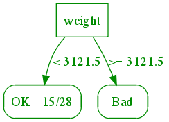
First level of the decision tree for the reduced auto MPG dataset
The root node represents the entire dataset, which has 19 bad, 15 OK, and 8 good examples (note that this is a subset of a much larger dataset that we also supply). As we consider each subcase at the leaves, the distribution of the subset of the data of bad/OK/good changes. Several leaves are "pure" -- they are all bad, OK, or good. For the mixed ones, we can further split them along different attributes as follows:

First two levels of the decision tree for the reduced auto MPG dataset
This might still not be enough, so let's continue until all leaves are pure. Note that this actually might not be possible, as you see in the un-splittable leaves below. In the un-splittable case, we predict whatever the majority of the outcomes is. For the leaves below 1 out of 2 of the leaves were "Bad"; we could have chosen the other result as well, but the code that generated the tree happened to choose "Bad" twice.
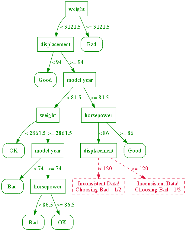
Complete decision tree with inconsistent data
Now we can use this organization of the data as a classifier. Given a new car with a set of attributes, we follow the splits from the root down to the leaf and return the majority label at that leaf as or prediction. In general, a decision tree maps an input {$\textbf{x}$} to a leaf of the tree {$leaf(\textbf{x})$} by following the path determined by the splits on individual features down to the leaf, where a distribution {$P(y\mid leaf(\textbf{x}))$} or simply the decision {$y(leaf(\textbf{x}))$} is defined.
Learning decision trees
There are many possible trees we can use to organize (i.e., classify) our data. It is also possible to get the same classifier with two very different trees. If we have a lot of features, trees can get very complex. Intuitively, the more complex the tree, the more complex and high-variance our classification boundary. Just like in linear models, we would like to control this complexity.
Let's assume for simplicity the there exists a tree that splits the data perfectly (all leaves are pure). A tree that splits the data with all pure leaves is called consistent with the data. This is always possible when no two samples {$(\textbf{x},y),(\textbf{x}',y')$} have different outcomes {$y\ne y'$} but identical features {$\textbf{x}=\textbf{x}'$}. Suppose we want to find the smallest (shortest) consistent tree. It turns out that this problem is NP-hard (Hyafil & Rivest, 76). We resort instead to a greedy heuristic algorithm:
Greedy Decision Tree Learning:
- Start from empty decision tree
- Split on next best feature (we'll define best below)
- Recurse on each leaf
Choosing what feature to split on
In order to choose what feature is best to split on for the above algorithm, we need to quantify how predictive a feature is for our outcome at the current node in the tree (which corresponds to the appropriate subset of the data). A standard measure of how much information a feature carries about the outcome is called information gain, and it's based on the notion of entropy. Recall that entropy of a discrete distribution {$P(Y)$} is a measure of uncertainty defined as:
{$\textbf{Entropy:}\;\; H(Y) = - \sum_y P(Y=y)\log_2 P(Y=y)$}.
A note about the notation: we write {$H(Y)$} when {$P(Y)$} is understood and unambiguous from the context. When it isn't, we will also need to specify which distribution on {$Y$} we mean.
For binary {$Y$}, the entropy is a function of {$p = P(Y=1)$}, {$H(Y) = - p\log_2 p - (1 - p)\log_2 (1-p)$} so we can plot it:
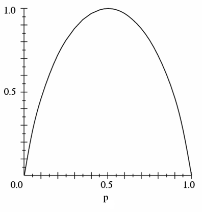
Entropy of a binary variable
Note that entropy is zero when p = 0 or p = 1, and 1 when p = 0.5. One interpretation of entropy is the expected number of bits needed to encode Y or questions needed to guess Y. E.g., an unbiased coin requires 1 bit, an eight sided die requires 3 bits, etc. However, if a coin is biased to always come up heads, it requires no bits to encode; regardless of what you do, it will always come up heads, so you don't need to encode anything.
Here is a heat map showing entropy of distributions over a ternary variable {$Y$}.
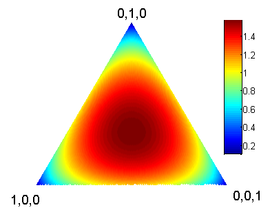
Entropy of a ternary variable
Each point in the triangle corresponds to a distribution {$(p_1,p_2,p_3)$}, where {$p_1+p_2+p_3=1$}. The corners correspond to the distributions that put all the weight on one of 3 outcomes (the entropy is zero there) and the center corresponds to the uniform distribution {$(\frac{1}{3},\frac{1}{3},\frac{1}{3})$} which achieves the entropy of {$1.585$}.
In order to quantify predictiveness of a feature X for Y, we consider the conditional entropy, or the expected number of bits needed to encode Y or questions needed to guess Y, knowing X. The conditional entropy of Y given X, H(Y|X), again assuming Y and X are discrete is defined as:
{$ Conditional Entropy: \begin{align*} H(Y|X) & = \sum_x P(X=x)H(Y|X=x) \\ & = -\sum_x P(X=x)\sum_y P(Y=y|X=x)\log_2 P(Y=y|X=x) \\ & = -\sum_{x,y} P(X=x,Y=y) \log_2 P(Y=y|X=x)\\ \end{align*} $}
So to measure the reduction in entropy of Y from knowing X, we use information gain:
{${\rm \textbf{Information Gain}:}\;\;\; IG(X) = H(Y)-H(Y|X)$}
For continuous variables, we can create splits by discretizing via introducing a thresholded feature {$X' = \mathbf{1}(X>\alpha)$} for some {$\alpha$} (this is not the only way, but perhaps the most common).
So our algorithm from above can be fleshed out now as:
Greedy Decision Tree Learning (based on ID3 algorithm by Quinlan, 1986):
- Start from empty decision tree
- Case 1: If all records in current data subset have the same output {$y$} then return leaf with decision {$y$}
- Case 2: If all records have exactly the same set of input attributes then return leaf with majority decision {$y$}
- Case 3 (Recursion): Split dataset on feature with best information gain and recurse on each branch with appropriate subset of the dataset
What if the best information gain is zero? Should we stop? Consider the same XOR function below.
| {$\mathbf{x_1}$} | {$\mathbf{x_2}$} | y |
|---|---|---|
| 1 | 1 | 0 |
| 0 | 0 | 0 |
| 1 | 0 | 1 |
| 0 | 1 | 1 |
which has the following graphical representation:
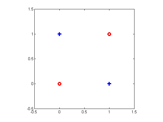
The information gain from either feature is zero, but the correct tree is:

The problem is that the information gain measure is myopic, since it only considers one variable at a time, so we cannot stop even if best IG=0.
Sample code
We will use the Sklearn decision tree package. If anyone wants matlab code, it is here.
Overfitting
Learning the shortest tree consistent with the data is one way to help avoid overfitting, but it may not be sufficient when the outcome labels are noisy (have errors). The lower we are in the tree, the less data we're using to make the decision (since we have filtered out all the examples that do not match the tests in the splits above) and the more likely we are to be trying to model noise. One simple and practical way to control data sparsity is to limit the maximum depth or maximum number of leaves. Another, more refined method, is decide for each split whether it is justified by the data. There are several methods for doing this, often called pruning methods, with chi-squared independence test being the most popular. Nilsson's chapter talks about several pruning methods, but we will not discuss these in detail.
Comparison to Nearest Neighbor
So why bother with decision trees at all when we have nearest neighbors? The answers are speed and size. When the dataset is large and has many dimensions, it can take a long time to decide which neighbor is closest (linear time in size of training data, naively, or, using faster using approximate methods). Although there are many methods to solve the problem, they are usually a lot slower than following a tree from root to leaf. This makes decision trees very attractive for large datasets. In addition to running time, nearest neighbors methods require storing the training data, which can be prohibitive for embedded systems. Another advantage is relative robustness to noisy or irrelevant features (assuming pruning or depth constraints).