Gaussians
Modeling continuous variables
The biased coin example involved discrete (Bernoulli) variables, and there was not much choice in modeling the probability distribution. When the number of outcomes is more than two or is continuous, there are many more choices. Besides the uniform distribution, the Gaussian distribution is perhaps the most (over) used distribution. For continuous variables that concentrate around the mean, like height, temperature, grades, or the amount of coffee in your cup every morning, the good old Gaussian is often a pretty decent start. Unfortunately, many phenomena are not as nice, but let's recall some basic properties.
The Gaussian Model
The univariate Gaussian distribution (aka the Normal distribution) is specified by mean {$\mu$} and standard deviation {$\sigma$}:
{$ p(x | \mu, \sigma) = \frac{1}{\sigma\sqrt{2\pi}} e^{\frac{-(x-\mu)^2}{2\sigma^2}} $}
Below are some examples, showing how the mean and standard deviation affect the shape of the distribution.
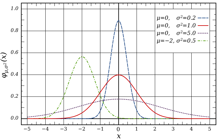
Example Gaussian distributions with different means and deviations
For the Gaussian distribution {$X \sim \mathcal{N}(\mu, \sigma^2)$}, we have mean and variance given by:
{$ \mathbf{E}[X] = \mu ;\;\;\;\;\;\; \mathbf{E}[(X - \mathbf{E}[X])^2] = \sigma^2$}
Gaussians behave nicely with linear transformations:
{$ Y = aX + b \; \rightarrow \; Y \sim \mathcal{N}(a\mu + b, a^2\sigma^2)$}
Sum of independent Gaussians {$X_i \sim \mathcal{N}(\mu_i, \sigma_i^2)$}:
{$ Y = \sum_i X_i \; \rightarrow \; Y \sim \mathcal{N}\left(\sum_i \mu_i, \sum_i \sigma^2_i\right)$}.
MLE for Gaussians
Assume our data are {$n$} i.i.d. samples from a Gaussian: {$D = \{x_1,\ldots,x_n\},\;\; X_i \sim \mathcal{N}(\mu, \sigma^2)$}. Let's derive MLE for the mean:
{$ p(D\mid\mu, \sigma) = \prod_i \frac{1}{\sigma\sqrt{2\pi}} e^{\frac{-(x_i-\mu)^2}{2\sigma^2}} $}
Taking logs:
{$ \log p(D\mid\mu, \sigma) = -n \log (\sigma \sqrt{ 2\pi}) - \sum_i \frac{(x_i-\mu)^2}{2\sigma^2} $}
Taking derivative with respect to {$\mu$} and setting it to zero:
{$ \sum_i \frac{x_i-\mu}{\sigma^2} = 0\;\;\; \rightarrow \hat\mu_{MLE} = \frac{1}{n}\sum_i x_i.$}
Taking derivative with respect to {$\sigma$} and setting it to zero:
{$ -\frac{n}{\sigma} + \sum_i \frac{(x_i-\mu)^2}{\sigma^3} = 0 \;\;\; \rightarrow \hat\sigma^2_{MLE} = \frac{1}{n}\sum_i (x_i - \mu)^2 = \frac{1}{n}\sum_i (x_i - \hat\mu_{MLE})^2.$}
No surprises here. One note is that the MLE variance estimate is biased, and most statistics book recommend using {${n-1}$} in the fraction instead -- we will define bias soon.
The Bayesian way
The conjugate prior for the mean of the Gaussian (with known variance) is a Gaussian. The conjugate prior for the variance of the Gaussian (with known mean) is Inverse Gamma, and if you want to have a prior on both, we can do that too, but don't worry about it (yet). Let's fix the variance and assume a Gaussian prior on the mean:
{$ p(\mu | \mu_0, \sigma_0) = \frac{1}{\sigma_0\sqrt{2\pi}} e^{\frac{-(\mu-\mu_0)^2}{2\sigma_0^2}} $}
Then the posterior is given by:
{$ \begin{align*}p(\mu | D, \mu_0, \sigma_0, \sigma) &= \frac{p(\mu, D | \mu_0, \sigma_0, \sigma)}{p(D | \mu_0, \sigma_0, \sigma)} \propto p(\mu, D | \mu_0, \sigma_0, \sigma) \\ &= p(\mu | \mu_0, \sigma_0) p(D | \mu, \sigma) \\ &= e^{\frac{-(\mu-\mu_0)^2}{2\sigma_0^2}} \prod_i e^{\frac{-(x_i-\mu)^2}{2\sigma^2}} \end{align*} $}
Note that if we combine all the exponents, we will get a quadratic in {$\mu$}, and we can rewrite the posterior in standard Gaussian form. Let's compute the MAP (which is the same as the posterior mean for the Gaussian case). Taking logs and setting the derivative to zero, we get:
{$-\frac{\mu-\mu_0}{\sigma_0^2} + \sum_i \frac{x_i-\mu}{\sigma^2} = 0 \;\;\; \rightarrow \;\; \hat\mu_{MAP} = \frac{\frac{\mu_0}{\sigma_0^2} + \sum_i \frac{x_i}{\sigma^2} }{\frac{1}{\sigma_0^2} + \frac{n}{\sigma^2} }$}
A few things to notice. First, MAP is a convex combination of prior mean and MLE mean. Second, as {$n\rightarrow\infty$}, {$\hat\mu_{MAP} \rightarrow \hat\mu_{MLE}$}. Third, when the prior is more uncertain, it matters less, that is {$\sigma_0 \rightarrow \infty, \;\;\hat\mu_{MAP} \rightarrow \hat\mu_{MLE}$}.