On this page… (hide)
There are many, many ways to interpret boosting: as exponential loss minimization, as a feature selection algorithm, as a kind of a game, … Historically, boosting was motivated by a theoretical question: suppose you have a black box which, given a binary classification dataset, always returned a classifier with training error strictly lower than 50% (this is called a weak classifier). Can one use it to build a strong classifier that has error close to 0? For example, my black box might be a decision tree learner that returns decision stumps or very short trees. Each tree is simple and usually underfits the data, and the goal of the boosting algorithm is to combine the trees to achieve small error.
The idea of combining different classifiers is often called ensemble learning. If the classifiers we are combining are all decent but different (i.e., make different, uncorrelated errors) than simple voting improves over each individual classifier since the errors cancel out. Boosting is often thought of as an ensemble method, where a set of binary classifiers, {$h_1(\mathbf{x}),\ldots,h_T(\mathbf{x})$} are combined by a weighted majority vote:
{$h(\mathbf{x}) = sign\left( \sum_{t=1}^T \alpha_t h_t(\mathbf{x}) \right)$}
(The sign function above is 1 when the argument is non-negative, and −1 otherwise.) The natural question is how to obtain decent but different classifiers? Boosting does this by reweighting the dataset before feeding it to the black box, essentially making certain examples more important to get right than others. Reweighting could be thought of as simply replicating certain examples proportionately to the weight in order to focus the classifier on predicting well on them.
The best algorithm to use on many data sets is Random forests, an ensemble method that combines decision trees; it is particularly widely used in medicine.
The AdaBoost algorithm is very simple: It iteratively adds classifiers, each time reweighting the dataset to focus the next classifier on where the current set makes errors.
Given: n examples {$(\mathbf{x}_i,y_i)$}, where {$\mathbf{x} \in \mathcal{X}, y \in \pm 1$}.
Initialize: {$D_1(i) = \frac{1}{n}$}
For {$t=1\ldots T$}
Output classifier: {$h(\mathbf{x}) = sign\left( \sum_{t=1}^T \alpha_t h_t(\mathbf{x})\right)$}
How do we set T? Cross-validation!
At iteration t, we obtain a classifier {$h_t(\mathbf{x})$}, whose weighted error is defined as:
{$\epsilon_t = \sum_i D_t(i) \mathbf{1}(y_i \ne h_t(\mathbf{x_i}))$}
Then a typical choice for {$\alpha_t$} (which you will partly derive in your homework) is:
{$\alpha_t = \frac{1}{2}\log\frac{1-\epsilon_t}{\epsilon_t}$}
Essentially, the weight of the classifier in the ensemble is proportional to the log-odds of it being correct vs making an error (assuming {$0<\epsilon_t<0.5$}). Below is a plot of the relationship:
Consider this toy dataset in 2D and assume that our weak classifiers are decision stumps (vertical or horizontal half-planes):
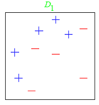
The first round:
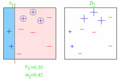
The second round:
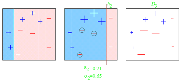
The third round:
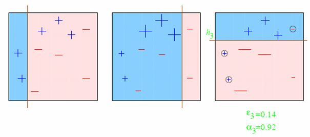
The final classifier
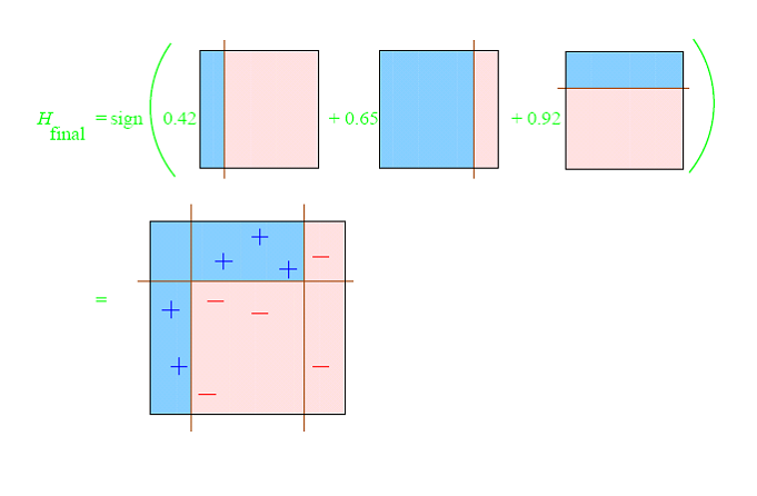
The reason behind the AdaBoost formulas for reweighing the data and weighing the classifiers is a key bound between error of the final classifier, {$h(\mathbf{x})$} and {$D_t,Z_t,\alpha_t$}. Let’s define:
{$f_\alpha(\mathbf{x}) = \sum_t \alpha_t h_t(\mathbf{x})$}
so that
{$h(\mathbf{x}) = sign(f_\alpha(\mathbf{x}))$}
After T rounds, the training error is bounded by:
{$\frac{1}{n} \sum_i \mathbf{1}(y_i \ne h(\mathbf{x}_i)) \leq \frac{1}{n} \sum_i \exp\{-y_i f_\alpha(\mathbf{x}_i)\} = \prod_{t=1}^T Z_t$}
where as before, {$Z_t = \sum_k D_t(k) \exp\{-\alpha_t y_k h_t(\mathbf{x}_k)\}$}. The first part of the bound, the inequality, is easy to see, {$\mathbf{1}(y_i \ne h(\mathbf{x}_i)) = \mathbf{1}(y_i f_\alpha(\mathbf{x}_i) < 0)$}:
The second part you can work out using recursion. The significance of this bound is that minimizing {$\prod_t Z_t$} in turn minimizes the training error and that’s exactly what AdaBoost is doing, one classifier at a time.
Assuming that we can keep learning weak classifiers on reweighted data with {$\epsilon_t < 0.5$}, you will derive the fact that the training error decreases exponentially fast:
{$\frac{1}{n} \sum_i \mathbf{1}(y_i \ne h(\mathbf{x}_i)) \leq \prod_{t=1}^T Z_t \leq \exp\{ \sum_t -2 (0.5-\epsilon_t)^2 \} \leq \exp\{-2T\gamma^2\}$}
where {$\gamma = \min_t (0.5-\epsilon_t)$}.
While it’s nice that training error is going down fast, it’s not the whole story. The interesting fact is that training error is not the best guide to test error. Consider this graph of training and test error taken from Schapire’s Tutorial
Test error keeps decreasing long after the training error has gone down to zero. One explanation is the margin, which takes into account the confidence of classification, not just the proportion of errors. How do we measure confidence of classification? In a probabilistic model, confidence is simply {$P(y_i\mid\mathbf{x}_i)$} (or it’s log). What about for a linear combination of classifiers? In order to measure confidence, we need a calibrated output, and for a weighted combination of classifiers, a natural notion of margin on an example i is:
{$\ell_1\textbf{-margin}: \;\; \frac{y_i f_\alpha(\mathbf{x}_i)}{||\alpha||_1}$}
called {$\ell_1$} because of the normalization by {$\ell_1$} norm of the weights. (We will see {$\ell_2$}-margin play a critical role in support vector machines soon.)
Essentially, the margin on each example is a measure how far from the decision boundary the example is, not just whether its on the correct side of the boundary. The farther an example is, the more confident the model is in its label, or another way of thinking about it, the decision is more robust to noise in the input features.
Recall the logistic regression maximizes {$\sum_i \log P(y_i|\mathbf{x}_i,\mathbf{w}) = \sum_i \log \frac{1}{1 + \exp(-y_i\mathbf{w}^\top\mathbf{x}_i)}$}, which is the same as minimizing {$\frac{1}{n}\sum_i \log (1 + \exp(-y_i\mathbf{w}^\top\mathbf{x}_i))$}. Let’s define, as for boosting:
{$f_\mathbf{w}(\mathbf{x}) = \mathbf{w}^\top\mathbf{x}$}
then looking at the two functions being minimized side by side, for each example:
{$\textbf{Boosting}:\;\; \exp(-y_i f_\alpha(\mathbf{x}_i)) \;\; \textbf{Logistic}: \;\; \log (1 + \exp(-y_if_\mathbf{w}(\mathbf{x}_i)))$}
If the set of possible classifiers is small, than we can just enumerate them all and learn using logistic. One difference would be that exponential loss is more sensitive to label noise (examples on the wrong side of the boundary). However, the key advantage of boosting is that we do not need to enumerate all classifiers, just to be able to find one good one on reweighted data. When the space of desired classifiers is very large, like all possible trees of a given depth with different possible threshold splits, boosting is the only way to learn in a reasonable amount of time. In applications where features are continuous (like computer vision, signal processing), boosting with very short trees is a classification method of choice.
Viola-Jones face detector is a very popular boosting-based classifier. (Or at least it was before deep learning came along.) It works by sliding a window over the image and deciding whether each window contains a face. Here is a perfect example:
Here is a slightly less perfect example:
The classifier uses boosting on top of the following Haar wavelets as basic features. (Again, something that is now found by deep learning.)
The first two features (wavelets) selected by boosting: