• View
• Edit
• History
• Print

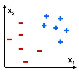
Classification

 

Classification

The goal of classification is to learn to predict a categorical outcome from input: for example, whether an email is spam or not, whether a patch of an image contains a face or not, is a news article about health or politics or technology, what zipcode number was scribbled on the envelope …

An email declared as spam by Gmail. The input can be represented as a set of features like counts of individual words in the email (bag-of-words model we’ll discuss later)

Face detection: a hard case. Inputs can be represented as simply the gray-scale values of individual pixels or gradients of gray-scale values or wavelet coefficients or …

As in regression, we have examples of inputs and outcomes {$(\mathbf{x}_i, y_i)$}, where the input is usually, as in regression, continuous features, {$\mathbf{x}\in R^m$}, but the outcome y is now discrete, one of K classes: {$y\in \{1,...,K\}$}. The simplest case is binary classification, when K = 2. In binary classification, we often call one class positive and the other negative (spam vs. non-spam) and encode the outcomes as {$y\in\pm 1$}. In the examples above, the input is very complex and high-dimensional, as is typical in machine learning problems, but here is a simple example of a classification problem with an input space is of dimension 2:

Example of binary classification problem in 2D.

Some inputs may not be real-valued but categorical to begin with, as in the example below, but we can transform them into real-valued features if needed. Suppose we want to predict what mode of transportation students will use on a given day (in order to manage traffic and parking, let’s say). Here is a small dataset with m=3 attributes and K=4 we might use to learn a model:

Abstractly, a classification algorithm takes as input a set of n i.i.d. examples {$D = \{\mathbf{x}_i, y_i\}$}, where {$\mathbf{x}\in \mathcal{X}$} and {$y\in \mathcal{Y}$} from an unknown distribution {$P(\mathbf{x},y)$} and produces a classifier {$h(\mathbf{x}): \mathcal{X} \mapsto \mathcal{Y}$} from a family of possible classifiers (called a hypothesis space, often denoted as {$\mathcal{H}$}). We will study several popular classification algorithms, including Naive Bayes, logistic regression, support vector machines, and boosting, but there are many more out there. The goal of a classification algorithm is usually to minimize expected classification error:

{$\textbf{Classification error of h:} \;\; \mathbf{E}_{(\mathbf{x},y)}[\textbf{1}(h(\mathbf{x}) \ne y)]$}

Generative vs. Discriminative Approaches

One of the main distinctions between classification algorithms is the Generative vs. Discriminative distinction: in a nutshell, generative classifiers focus on modeling {$P(\mathbf{x},y)$} and discriminative algorithms focus on {$P(y \mid \mathbf{x})$}.

Generative approach

The idea behind generative approaches is simple: estimate {$\hat{P}(\mathbf{x},y)$} from examples (say using MLE) and then produce a classifier:

{$h(\mathbf{x}) = \arg\max_y \hat{P}(y\mid \mathbf{x}) = \arg\max_y \frac{\hat{P}(\mathbf{x},y)}{\sum_{y'}\hat{P}(\mathbf{x},y')} $}

For binary classification, this reduces to:

{$h(\mathbf{x}) = \left\{ \begin{array}{ll} 1 & \textrm{if} \;\;\; \hat{P}(\mathbf{x}, 1) \ge \hat{P}(\mathbf{x},-1) \\ -1 & \textrm{otherwise} \end{array} \right. $}

If we are (very) lucky and we learn a perfect model of the data {$\hat{P}(\mathbf{x}, y) = P(\mathbf{x}, y)$}, the above classifier is optimal (it’s called Bayes optimal) in a sense that no other classifier can have lower expected classification error. However {$P(\mathbf{x},y)$} is usually very complex: think of trying to model a distribution over images or email messages. The Naive Bayes model, which we will discuss next, makes a very simple approximation to {$P(\mathbf{x},y)$} that nevertheless often works well in practice.

Discriminative approach

Because the joint distribution {$P(\mathbf{x},y)$} could be very complex, discriminative approaches try to circumvent modeling it and focus on modeling {$P(y\mid\mathbf{x})$} directly, (especially in parts of the space where {$P(\mathbf{x})$} is large). Logistic regression, as we’ll discuss soon, models {$P(y\mid\mathbf{x})$} as log-linear and then attempts to estimate parameters {$\textbf{w}$} using MLE or MAP. More generally, discriminative methods like SVMs and boosting focus directly on learning a function {$h(\textbf{x})$} that minimizes expected classification error, without any probabilistic assumptions about {$P(\mathbf{x},y)$}.

Back to Lectures