• View
• Edit
• History
• Print

TA Notes 2

 

1.  Perspective on the Last Few Weeks

We’ve looked at several different types of models, where by “model” we mean an equation that attempts to describe how some data was generated:

All of these models are probabilistic. For any probabilistic model, our goal is always to maximize probability by setting the parameters appropriately; that is, the parameter estimation method is: {$\arg\max_{\textrm{params}} \textrm{formula}$}

We call this procedure maximizing the likelihood. For the simple models we’ve seen so far, all except logistic regression have a closed form parameter estimate; that is, taking the derivative of the model likelihood and setting it equal to zero, we’ve been able to get a formula for the parameters. We’ve also considered all of these methods from a Bayesian perspective, which just means that we’ve incorporated some prior knowledge into the models to reflect original beliefs we might have about the parameters. For example, in the biased coin model we incorporated prior knowledge by saying “most coins I’ve seen in my life are fair”, so we assumed that the probability of heads was drawn from a {$Beta$} distribution peaked around the value {$1/2$} (chance of flipping heads equals chance of flipping tails). Then, instead of maximizing just the likelihood to estimate our parameters, we multiplied the likelihood by the prior and maximized this quantity, which we called the maximum a posteriori (MAP) estimate. The table below lists the type of all the parameter priors for the models we’ve considered so far:

We can also compare these methods according to some other important attributes:

The next few sections below clarify a few points from class.

2.  Names: Generative vs. Discriminative

We call learning methods that model the full joint {$P(x,y)$} “generative” and methods that model just the conditional {$P(y \mid x)$} “discriminative”. Why does “generative” mean modeling full joint and “discriminative” mean modeling just the conditional? Where did these names come from?

Well, consider the generative case, where we have some model of the joint {$P(x,y)$}. Given such a model, we are able to “generate” values of either {$x$} or {$y$}. For example, suppose our model is {$P(X,Y \mid \mu_1, \sigma_1, \mu_2, \sigma_2)$} where our data comes from 2 Gaussians, one for {$Y = 1$} and one for {$Y = -1$}. If we wanted to generate more points for these Gaussians using our model, we could easily generate new {$(x,y)$} pairs by drawing from the joint distribution. But if we just had the conditional {$P(Y \mid X, \mu_1, \sigma_1, \mu_2, \sigma_2)$} as in the discriminative case, then we can generate new {$y$}, but not new {$(x,y)$} pairs. Thus, the conditional model is just “discriminative”, in that it can discriminate between different values of the output {$y$}, though it can’t be used to generate {$(x,y)$} pairs.

3.  Large Weights Mean High Variance

In class we derived bias and variance definitions for the general case of observing i.i.d. samples from any probability distribution. Let’s take a closer look at what bias and variance mean for linear regression. Recall that for linear regression we’re trying to make {$y = \textbf{w}^\top\textbf{x}$} by setting {$\textbf{w}$} appropriately. Suppose we have some setting for {$\textbf{w}$}, and consider the derivative {$\frac{\delta y}{\delta x_i} = w_i$}. If you have high weights, this derivative is large. A large derivative means the function changes rapidly with {$x$}. Rapid change with {$x$} means that given a new data point, our model may be far from correct for this new point. So, large weights mean that the difference {$h(x;D) - \bar{h}(x)$} can be very large. This makes variance {$\textbf{E}_{x,D}[ (h(x;D) - \bar{h}(x))^2]$} large.

4.  Linear Regression vs. Logistic Regression

In the first TA notes we distinguished “regression” as a learning method that predicts a {$Y \in \mathbb{R}$}. Though this is the most common use, “regression” is actually a more general term that really just means modeling the relationship between a dependent variable ({$Y$}) and some inputs ({$X$}). In class we have considered both “linear regression” which predicts a {$Y \in \mathbb{R}$}, and “logistic regression” which predicts a {$Y \in \{1, \ldots, K\}$} (K-class classification). Both of these methods produce a linear decision boundary, so it’s a logical question to ask why we didn’t just threshold the linear regression output to produce a classifier, instead of creating this whole other logistic method. That is, instead of deriving this whole new logistic regression method with this complicated formula {$P(Y=y_k|\textbf{x},\textbf{w}) = \frac{\exp\{-\textbf{w}_k^\top \textbf{x}_k\}}{\exp\{-\sum_k w_k^\top x_k\}}$}, why not just take linear regression’s formula {$y = \textbf{w}^\top \textbf{x}$} and wrap it in a function {$g$} that only takes on the values {$\{1, \ldots, K\}$}. For example, consider the two-class case with {$Y \in \{-1, 1\}$}:

{$ y = g(\textbf{w}^\top \textbf{x}) = \begin{cases} 1 & \textrm{if}\;\; \textbf{w}^\top \textbf{x} > 0 \\ -1 & \textrm{if}\;\; \textbf{w}^\top \textbf{x} < 0 \end{cases} $}

At first glance, this seems like a reasonable way to create a classifier. However, there is a potential problem with this approach: if we estimate {$\textbf{w}$} in the same way as for normal linear regression, then we’re minimizing the following sum of squared errors over our training data: {$\sum_i (y_i - \textbf{w}^\top \textbf{x}_i)^2.$} What can go wrong here? First, note that {$y \in \{-1, +1\}$}. Suppose that {$\mathbf{w}^\top\mathbf{x} = 5$}, and {$y = 1$}. Is this a mistake? No, because {$g(5) = \mathrm{sign}(5) = +1$}. But the squared error in fact penalizes this term, since {$(y - \mathbf{w}^\top\mathbf{x})^2 = (1 - 5)^2 = 16$}. In other words, the squared error will penalize very confident correct guesses from the linear regression! This is an example of using an inappropriate loss function, where the loss function is actually working against us.

Another problem can be demonstrated as follows. If we have data that looks like that below, the linear regression approach would be ok: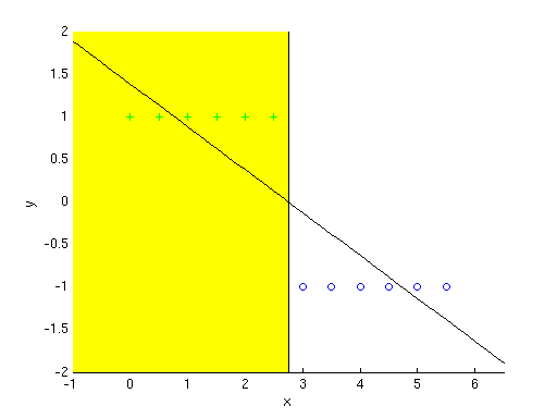

Positive examples are green plus signs, negative examples are blue circles. The learned classifier is {$y = g(-0.5035x + 1.3846)$} (diagonal line) which means for all x in the portion of the graph that’s highlighted yellow, the classifier predicts positive +. Seems pretty good, no?

But now suppose our data includes an outlier point, like the one at {$x = 15$}. Then the classifier that linear regression learns for this data is shown by the dotted line, which makes mistakes in the region highlighted in red below.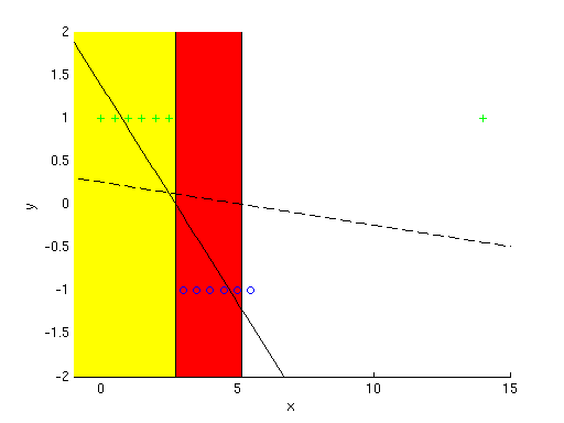

The addition of an outlier data point changes the classifier we learn to the dotted line, putting it’s cutoff value past many of the negative examples, which are then misclassified.

So, as this example shows, using a thresholded version of linear regression gives undue consideration to outliers, because it minimizes {$\sum_i (y_i - \textbf{w}^\top \textbf{x}_i)^2$}.

You might ask, we built a classifier using {$g(\textbf{w}^\top \textbf{x})$}, so why are we not including it in the objective that we’re minimizing? Would that not fix both of these problems? In other words, what if we minimized the quantity, {$\sum_i (y_i - g(\textbf{w}^\top \textbf{x}_i))^2.$}

The problem with this is that {$g(\textbf{w}^\top \textbf{x}_i)$} is not differentiable, and makes the objective non-convex, so we can’t easily find the maximum. In fact, we can’t even find the gradient, so we can’t do what logistic regression does and follow the gradient to find the maximum. For these reasons, we turn to logistic regression to do classification instead of just trying to threshold linear regression.

That being said, there are caveats to this. Although we cannot find the gradient of the above loss function, we can still find directions to move iteratively that act kind of like a gradient would to a certain extent. This also brings up a topic we’ll discuss later in the class when we get to neural networks and support vector machines. For example, an alternative to using logistic regression would have been to use the perceptron classifier. The perceptron classifier essentially optimizes exactly the error function that we described above, but it does so incrementally, using one example at a time to update the weights with a simple equation. That sort of learning (picking up one example at a time) is known as online learning. We may not have time to cover this in much detail in the course, but you can use the online algorithm Wikipedia page as a starting point if you’re interested to know more about this topic.