Recitation Remix 2012On this page… (hide) 1. Linear boundary for 2-class Gaussian Naive Bayes with shared variancesFor Gaussian Naive Bayes, we typically estimate a separate variance for each feature j and each class k, {$\sigma_{jk}$}. However consider a simpler model where we assume the variances are shared, so there is one parameter per feature, {$\sigma_{j}$}. What this means is that the shape (the density contour ellipse) of the multivariate Gaussian for each class is the same. In this case the decision boundary is linear: {$P(Y=1|X) = \frac{1}{1 + \exp\{w_0 + \textbf{w}^\top X\}}, \; {\rm for}\;\; {\rm some} \;\; w_0,\textbf{w}$} Let’s derive it: {$ \begin{align*} P(Y=1|X) & = \frac{P(Y=1)P(X|Y=1)}{P(Y=1)P(X|Y=1)+P(Y=0)P(X|Y=0)}\\ & = \frac{1}{1+\frac{P(Y=0)P(X|Y=0)}{P(Y=1)P(X|Y=1)}}\\ & = \frac{1}{1+ \exp\Big(\log \frac{P(Y=0)P(X|Y=0)}{P(Y=1)P(X|Y=1)}\Big)} \end{align*} $} Now let’s plug in our definitions: {$ \begin{align*} P(Y=1) & =\theta \\ P(X_j|Y=1) & = \frac{1}{\sigma_j\sqrt{2\pi}} \exp\Bigg\{\frac{-(X_j-\mu_{j1})^2}{2\sigma_j^2}\Bigg\}\\ P(X_j|Y=0) & = \frac{1}{\sigma_j\sqrt{2\pi}} \exp\Bigg\{\frac{-(X_j-\mu_{j0})^2}{2\sigma_j^2}\Bigg\} \end{align*} $} Note that here we’re using capital {$X$} and {$X_j$} to denote that these are random variables (and not to imply that they are matrices). We now have: {$ \begin{align*} & \log \frac{P(Y=0)P(X|Y=0)}{P(Y=1)P(X|Y=1)} \\ & = \log P(Y=0) + \log P(X|Y=0) - \log P(Y=1) - \log P(X|Y=1)\\ & = \log \frac{P(Y=0)}{P(Y=1)} +\sum_j\log\frac{P(X_j|Y=0)}{P(X_j|Y=1)} \end{align*} $} Question: How did we get to the previous step in this derivation? What assumptions did we have to make?
We use the “naive” assumption of the Naive Bayes model. That is, we say the features are conditionally independent, given the label: (:centereq:) {$\hat{P}(\mathbf{X}\mid Y) = \prod_j \hat{P}(X_j\mid Y) $} (:centereqend:) In general, it is not necessarily true that the features are conditionally independent if we know the label. However, this assumption allows us to greatly simplify our class model. Let’s examine the {$ \sum_j\log\frac{P(X_j|Y=0)}{P(X_j|Y=1)} $} term. By plugging in our definitions, we get: {$ \; $ \begin{align*} \sum_j\log\frac{P(X_j|Y=0)}{P(X_j|Y=1)} =& \sum_j \log\left( \frac{\frac{1}{\sigma_j\sqrt{2\pi}}\exp\left(\frac{-(X_j-u_{j0})^2}{2\sigma_j^2} \right)}{\frac{1}{\sigma_j\sqrt{2\pi}}\exp\left(\frac{-(X_j-u_{j1})^2}{2\sigma_j^2} \right)} \right)\\ =&\sum_j \log\left[ \exp\left(-\frac{(X_j-u_{j0})^2}{2\sigma_j^2} + \frac{(X_j-u_{j0})^2}{2\sigma_j^2} \right)\right]\\ =& \sum_j \frac{-X_j^2 + 2X_j\mu_{j0} -\mu_{j0}^2 + X_j^2 - 2X_j\mu_{j1}+\mu_{j1}^2}{2\sigma_j^2} \end{align*} $ \; $} Now we substitute it back into the original equation: {$ \begin{align*}& = \log \frac{1-\theta}{\theta} + \sum_j \frac{(\mu_{j0} - \mu_{j1})X_j}{\sigma_j^2} + \frac{\mu_{j1}^2 - \mu_{j0}^2}{2\sigma_j^2}\\ & = w_0 + \textbf{w}^\top X\end{align*} $} Question: What can we say about the decision boundary for GNB with shared variances? Since the decision boundary has the same parametric form as that for logistic regression, it will also be a linear decision boundary. Question: Does this mean that GNB with shared variances and logistic regression will find the same decision boundary on a given problem? No. Remember that the fitting process for GNB is different than that for logistic regression. For logistic regression, we maximize the conditional likelihood of the labels given the data: (:centereq:) {$\log P(\mathbf{Y}\mid\mathbf{X}) = \sum_i \log P(y_i \mid \mathbf{x}_i)$} (:centereqend:) For GNB, we maximize the joint likelihood of the labels and the data: (:centereq:) {$\log P(\mathbf{Y}, \mathbf{X}) = \sum_i \log P(y_i,\mathbf{x}_i) = \sum_i \log P(y_i) + \log P(\mathbf{x}_i \mid y_i)$} (:centereqend:) Question: Why do we need to use shared variances to get a linear decision boundary? If we did not use shared variances, then in the above derivation we would be left with an {$X_j^2$} term, making the decision boundary quadratic. 2. LOO: Leave-one-out cross-validationWhen the dataset is very small, leaving one tenth out depletes our data too much, but making the validation set too small makes the estimate of the true error unstable (noisy). One solution is to do a kind of round-robin validation: for each complexity setting, learn a classifier on all the training data minus one example and evaluate its error the remaining example. Leave-one-out error is defined as: {$\textbf{LOO error}: \frac{1}{n} \sum_i \mathbf{1}(h(\mathbf{x}_i; D_{-i})\ne y_i)$} where {$D_{-i}$} is the dataset minus ith example and {$h(\mathbf{x}_i; D_{-i})$} is the classifier learned on {$D_{-i}$}. LOO error is an unbiased estimate of the error of our learning algorithm (for a given complexity setting) when given n-1 examples. Intuitively, LOOCV is cross validation with the number of folds set to the number of training points. Question: Suppose we train a set of weights {$ \hat{w}^{(-i)} $} on a data matrix that has one example removed, denoted by {$ X^{(-i)} $}. We then make a prediction using the trained weights: {$\hat{Y}^{(-i)} = X\hat{w}^{(-i)}$}. What is the dimensionality of {$ \hat{Y}^{(-i)} $}? Event though we have trained {$ \hat{w}^{(-i)} $} on {$ X^{(-i)} $}, the dimensionality of {$ \hat{w}^{(-i)} $} is still mx1. We have one weight for each feature, not each data point. Therefore, the dimensionality of {$ \hat{Y}^{(-i)} $} is nx1. 3. MLE Examples3.1 Poisson distributionThe Poisson distribution can be useful to model how frequently an event occurs in a certain interval of time (packet arrival density in a network, failures of a machine in one month, customers arriving at a waiting line…). Like any other distribution, the parameter (here {$\lambda$}) can be estimated from some measurements/experiences. The pmf is the following: {$P(X \mid \lambda) = \frac{\lambda^X e^{-\lambda}}{X!}$}
3.2 Multivariate Gaussian EstimationThe formula for the multivariate Gaussian is much like that of the univariate Gaussian. Consider the n-variate case where {$X = (X_1, X_2, \ldots, X_n)$}: {$ P(X \mid \mu, \Sigma) = \frac{1}{(2\pi)^{n/2} |\Sigma|^{1/2}} \exp \Bigg(-\frac{1}{2} (X - \mu)^T \Sigma^{-1}(X - \mu) \Bigg). $} {$\Sigma$} is called the covariance matrix. Expanding all the vectors and matrices in this formula to clarify what each contains: {$ P\left( \left.\left[ \begin{array}{c} X_1 \\ \vdots \\ X_n \end{array} \right]\;\; \right\vert \;\; \left[ \begin{array}{c} \mu_1 \\ \vdots \\ \mu_n \end{array} \right], \left[ \begin{array}{ccc} \sigma_{11} & \ldots & \sigma_{1n} \\ \vdots & \vdots & \vdots \\ \sigma_{n1} & \ldots & \sigma_{nn} \end{array} \right] \right) = (2\pi)^{-n/2} \left| \begin{array}{ccc} \sigma_{11} & \ldots & \sigma_{1n} \\ \vdots & \vdots & \vdots \\ \sigma_{n1} & \ldots & \sigma_{nn} \end{array} \right|^{-1/2} e^{\Omega}$} where {$\Omega = \Bigg(-\frac{1}{2} \left[ \begin{array}{ccc} (X_1 - \mu_1) & \ldots & (X_n - \mu_n) \end{array} \right] \left[ \begin{array}{ccc} \sigma_{11} & \ldots & \sigma_{1n} \\ \vdots & \vdots & \vdots \\ \sigma_{n1} & \ldots & \sigma_{nn} \end{array} \right]^{-1} \left[ \begin{array}{c} X_1 - \mu_1 \\ \vdots \\ X_n - \mu_n \end{array} \right] \Bigg)$} where {$\sigma_{ij} = cov(X_i, X_j) = \mathbb{E}_X[(X_i - \mu_i)(X_j - \mu_j)]$}, hence {$\sigma_{ii} = var(X_i) = \mathbb{E}_X[(X_i - \mu_i)^2]$}. In the exercises below, we’ll consider how to best set the parameters of a bivariate Gaussian, {$P(X_1, X_2 \mid \mu_1, \mu_2, \sigma_{11}, \sigma_{22}, \sigma_{12})$}, on the basis of a dataset {$D = \left\{(x_{1}^{(1)}, x_{2}^{(1)}), \ldots, (x_{1}^{(m)}, x_{2}^{(m)})\right\} $} which contains {$m$} data points.
(:answiki:) We will show the result for the multivariate case and interpret it in the 2D case. Just like in the 1D case, the procedure is the following:
Here the parameters we want to estimate are a vector ({$\mu$}) and a matrix ({$\Sigma$}). We could develop the likelihood to expose {$\mu_1,\mu_2,\sigma_{11},\sigma_{22},\sigma_{12}$} and take derivatives w.r.t. each of them, but let’s use a faster method: we are going to take derivatives with respect to the vector {$\mu$} and the matrix {$\Sigma$}:
Here are useful derivation formulas that we will use. Make sure you understand the dimensions using the 3 facts above. When {$x$} is a vector and {$A$} and {$B$} squared matrices, we have:
MLE of the mean (:centereq:) {$\begin{array}{rl} \log P(D \mid \mu,\Sigma) &= -\frac{Nd}{2} \log(2\pi) - \frac{N}{2} \log |\Sigma| - \frac{1}{2} \sum_{i=1}^N (x_i-\mu)^T \Sigma^{-1}(x_i-\mu) \\ \frac{d\log P(D \mid \mu,\Sigma)}{d\mu} &= \sum_{i=1}^N (x_i-\mu)^T \Sigma^{-1} \end{array}$} (:centereqend:) By setting this derivative to zero (which means we are setting all its components to 0, since it is a vector), we have the following: (:centereq:) {$\mu_{MLE} = \frac{1}{N} \sum_{i=1}^N x_i$} (:centereqend:) MLE of the variance (:centereq:){$\frac{d\log P(D \mid \mu,\Sigma)}{d(\Sigma^{-1})} = 0 = \frac{N}{2}\Sigma - \frac{1}{2}\sum_i (x_i-\mu)(x_i-\mu)^T$}(:centereqend:) (:centereq:) {$\Sigma_{MLE} = \frac{1}{N} \sum_i (x_i- \mu)(x_i - \mu)^T$} (:centereqend:) This turns out to be the empirical covariance matrix of the data: we will study its properties and meaning later on, when we will introduce PCA. Using the two MLE formulas we just found, we can write the coefficients of {$\mu$} and {$\Sigma$} in 2D as follows: (:centereq:) {$ \begin{array}{rl} \hat{\mu}_{1_{MLE}} & = \frac{1}{m} \sum_{i = 1}^m x_1^{(i)} \\ \hat{\sigma}_{11_{MLE}} & = \frac{1}{m} \sum_{i = 1}^m (x_1^{(i)} - \hat{\mu}_1)^2 \\ \hat{\sigma}_{12_{MLE}} & = \frac{1}{m} \sum_{i = 1}^m (x_1^{(i)} - \hat{\mu}_1)(x_2^{(i)} - \hat{\mu}_2) \end{array} $} (:centereqend:) (:answikiend:)
The intermediate steps are not shown here, but the general procedure is to form the likelihood*prior, {$\prod_{i = 1}^m P_i*P(\mu)$}, where each {$P_i$} is in the form of a bivariate Gaussian, then take the log of this expression to make the math easier later, then take the derivative with respect to {$\mu_1$}, then set that equal to 0, and finally solve for {$\mu$}. (:centereq:) {$ \hat{\mu}_{MAP} = (\Sigma_0^{-1} + m\Sigma^{-1})^{-1}\Bigg(\mu_0^T\Sigma_0^{-1} + \sum_{i = 1}^m x^{(i)}\Sigma^{-1}\Bigg) $} (:centereqend:) where {$\mu_0 = [\mu_{1_0}, \mu_{2_0}]^T$} and {$x^{(i)} = [x_1^{(i)}, x_2^{(i)}]^T$} (the i-th data point). (:ansend:) MLE for the general multivariate case is detailed on Wikipedia, if you’re curious. 3.3 Poisson distributionThe Poisson distribution can be useful to model how frequently an event occurs in a certain interval of time (packet arrival density in a network, failures of a machine in one month, customers arriving at a waiting line…). Like any other distribution, the parameter (here {$\lambda$}) can be estimated from some measurements/experiences. The pmf is the following: {$P(X \mid \lambda) = \frac{\lambda^X e^{-\lambda}}{X!}$}
4. Basis functionsEven though LR and sometimes GNB result in linear decision boundaries, we can still potentially learn very difficult, non-separable datasets by transforming the inputs using basis functions. For example, consider the XOR dataset: 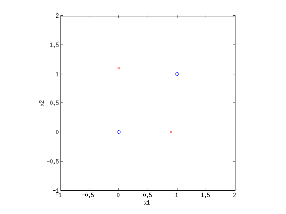 Clearly this is not separable. But by transforming the input into a new space, this dataset can be made separable. Consider {$\phi_1(\mathbf{x}) = x_1+x_2$} and {$\phi_2(\mathbf{x}) = x_1\cdot x_2$}. If we plot the same data along the new dimensions {$\phi_1$} and {$\phi_2$}, we find: 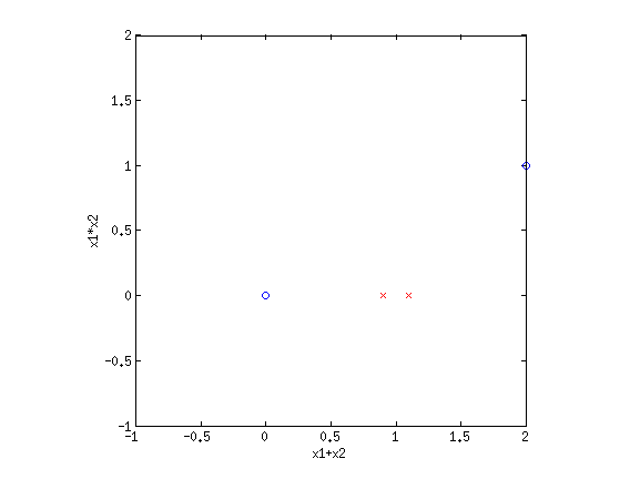 The data is now separable! Let’s look at another example. 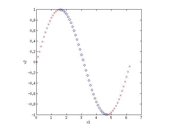 This looks like a sin function, and it is also not separable. However, if we could “flip” the orientation of the curve, we could draw a line through the data. Let’s consider the new basis {$\phi_1(\mathbf{x}) = x_1$} and {$\phi_2(\mathbf{x}) = \cos x_1$}: 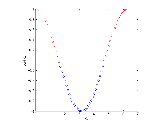 Now we have once again transformed a non-linearly separable dataset into one that is linearly separable. 4.1 Practice problemsWhat basis functions could we use to make the following datasets linearly separable? 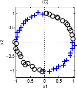
One way to transform this is to notice that the quadrants where {$\mathrm{sign}\left(x_1\right) = \mathrm{sign}\left(x_2\right)$} are the same class. Therefore we could use a single basis function {$\phi(\mathbf{w}) = x_1 \cdot x_2$}, and would separate this data along a single line. 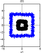
Again, we can use a single basis function: {$\phi(\mathbf{x}) = ||\mathbf{x}||_2$}, since the inner class is closer to the center (and therefore smaller norm) than the outer class. 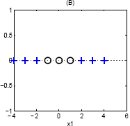
Consider the basis, {$\phi_1(\mathbf{x}) = x_1, \phi_2(\mathbf{x}) = x_1^2$}. This will raise the line into a parabola, with the top of the parabola being separable from the bottom half. These are all carefully constructed toy examples, but the point is to demonstrate that determining what is linearly separable is not an easy question. As the saying goes, one man’s garbage is another man’s linearly separable dataset. |