• View
• Edit
• History
• Print

PCA Prep

 

Why EM

In class we saw that Gaussian EM is a generalization of k-means. We began from the iterative algorithm for k-means:

1. Assign points to k clusters (say, randomly at first).
2. Compute the means of these clusters.
3. Iterate --- assign each point to the cluster whose mean is closest to that point, then recompute the means, continuing until the cluster assignments stabilize.

From there we considered the generalization in which a point can be a partial member of many clusters. We defined an iterative algorithm similar to the k-means algorithm where the main difference is just that the step “assign points to clusters” is replaced by a soft assignment in which we determine the probability that a point belongs to each cluster. We called this algorithm “Gaussian EM”, with the “assign the points” step re-named the “E-step” (expectation step) and the “compute the means” step re-named the “M-step” (maximization step).

However, we also noted that what the EM algorithm is really doing is attempting to find a maximum of the following marginal likelihood objective:

{$\begin{array}{rcl} \log P(D \mid \pi,\mu,\Sigma) & = & \sum_i \log \sum_k p_\pi(z_i=k) p_{\mu,\Sigma}(\mathbf{x}_i \mid z_i=k) \\ & = & \sum_i \log \sum_k p_\pi(z_i=k) N(\mathbf{x}_i ; \mu_k,\Sigma_k) \end{array}$}

and that it is only guaranteed to find a local maximum, not a global maximum. In other words, the iterative procedure inspired by k-means finds a local maximum of the above objective. This is distinct from the types of optimization procedures we’ve used before, such as naive Bayes or logistic regression or SVMs, in two ways:

1. We only achieve a local maximum of the objective.
2. We get to this local maximum not by using closed-form formulas (like for naive Bayes), or by using gradient ascent on all variables in each ascent step (like for logistic regression), or by using a quadratic program solver (like for SVMs), but rather by doing coordinate ascent.

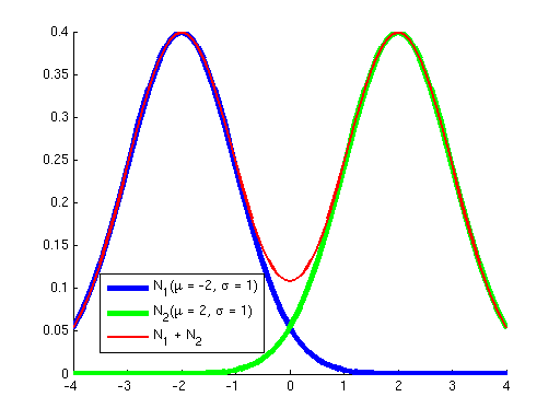
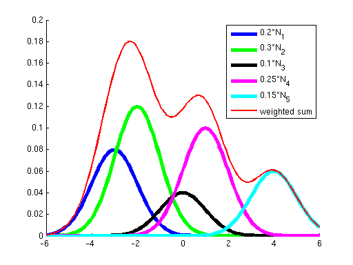
Let’s address each of these points in turn.

Only a Local Optimum

First, why did we learn a procedure for finding a local optimum instead of a global optimum? The answer is that for all the problems we’ve seen before, the objective has been convex; it has not had any local optima, so methods like gradient ascent that “hill-climb” only had a single hill to climb --- once they got to the top (where the derivative of the objective is approximately zero), we knew that we had reached the global optimum. However, the objective optimized by Gaussian EM is not convex; it has many local optima. To see this, consider the two graphs below. The graph on the left shows in blue two Gaussians and in red the sum of these two. While each of the Gaussians has a single peak, their sum has multiple peaks. Similarly, the graph on the right shows a sum of five Gaussians, where additionally each Gaussian has a weight. (Weights correspond to the {$p_{\pi}(z_i=k)$} terms in the objective.) You can see how as the number of Gausssians increases we can get a more complex landscape with many hills of differing heights.

Sum of 2 Gaussians.	Sum of 5 weighted Gaussians.

For those who are familiar with the properties of convexity, here’s a 1-sentence explanation of why the objective is not convex: The Gaussian distribution is log-concave, and the product of log-concave functions is concave, but their sum is not.

Inefficiency of Gradient Ascent

Reconciled to the fact that finding a global optimum may be hard, how can we at least climb one hill to reach a local optimum? Why not just do gradient ascent on all the variables at the same time, like we saw for logistic regression? We could in fact do this. However, the procedure would most likely be more computationally expensive than the iterative EM algorithm. Here’s what the gradient ascent procedure would look like:

1. Start from some (possibly random) initial setting of all the variables
2. Compute the gradient with respect to each variable
3. Search for an appropriate step size (learning rate)
4. Take a step: new variable value = old variable value + (step size) * gradient
5. Loop back to step 2 until the gradient is almost zero

This is more expensive than EM in two ways:

1. EM has closed-form expressions for setting the variables each E-step and M-step, which are likely cheaper to compute than the expressions for all the gradients.
2. EM does not require a search for step size; searching for step size means having to repeatedly compute the value of the objective.

So, because we like efficiency, EM is the procedure of choice for optimizing the {$\log P(D \mid \pi,\mu,\Sigma)$} objective shown above.

Linear Algebra Review (PCA Preparation)

In the previous lecture, we introduced principal components analysis (PCA). The point of PCA is dimensionality reduction, mapping from a high-dimensional space to a low-dimensional space. This is useful for several reasons:

1. In a lower-dimensional space, many algorithms may run faster.
2. In very low dimensions, such as 2D or 3D space, we can plot the data and get a good visual intuition about its characteristics (e.g. are there 10 clusters of points? 20 clusters? etc.).

Recall from lecture that the procedure for preforming PCA is:

• Given {$D = \mathbf{x}^1, \ldots, \mathbf{x}^n$}
• Compute {$\mathbf{\overline x} = \frac{1}{n}\sum_i\mathbf{x}^i$} and {$\Sigma = \frac{1}{n}\sum_{i=1}^n (\mathbf{x}^i-\mathbf{\overline x}) (\mathbf{x}^i-\mathbf{\overline x})^\top$}
• Find k eigenvectors of {$\Sigma$} with largest eigenvalues: {$\mathbf{u}_1,\ldots,\mathbf{u}_k$}, called principal components.
• Project: {$ \mathbf{z}^i = \left( (\mathbf{x}^i-\mathbf{\overline x})^\top\mathbf{u}_1, \ldots,(\mathbf{x}^i-\mathbf{\overline x})^\top\mathbf{u}_k \right)$}

To give an intuition as to why the top k eigenvectors of {$\Sigma$} are “good” dimensions to project down onto, we will show that these eigenvectors define the directions along which the data has greatest variance. If we project down to these dimensions, we will have captured as much of the data’s variance as it is possible to capture in k dimensions. Before proving the eigenvectors of {$\Sigma$} are “good”, let’s start by briefly recalling a few basics about vectors, matrices, and how to compute eigenvalues.

Vector Basics

For {$m$}-dimensional vectors {$\mathbf{v}$} and {$\mathbf{u}$} that form angle {$\theta$} with each other:

Property Name	Denotation	Formula
Length of {$\mathbf{v}$}	{$|\mathbf{v}|$} or {$||\mathbf{v}||_2$}	{$\sqrt{\sum_{i = 1}^{m} v^2_i}$}
Inner (dot) product of {$\mathbf{v}$} and {$\mathbf{u}$}	{$\mathbf{v} \cdot \mathbf{u}$} or {$\mathbf{v}^T \mathbf{u}$} or {$<\mathbf{v}, \mathbf{u}>$}	{$\sum_{i = 1}^m v_i u_i$} or {$|v||u|\cos(\theta)$}
Projection of {$\mathbf{v}$} onto {$\mathbf{u}$}	{$\textrm{proj}_{\mathbf{u}}(\mathbf{v})$}	{$<\mathbf{v},\mathbf{u}> \frac{\mathbf{u}}{<\mathbf{u},\mathbf{u}>}$}

Vectors of unit length ({$|\mathbf{v}| = 1$}) are called normal vectors. Two vectors {$\mathbf{v}$} and {$\mathbf{u}$} are said to be orthogonal, {$\mathbf{v} \perp \mathbf{u}$}, if {$\mathbf{v} \cdot \mathbf{u} = 0$}. In {$2D$} this corresponds to them being at a {$90^\circ$} angle. Two normal vectors that are orthogonal are called orthonormal. You can get a geometric intuition for the dot product and orthogonality by playing with this dot product applet. Note that for the purposes of multiplication, it’s convention to assume vectors are vertical, and that their transposes are horizontal as shown below.

{$\mathbf{v} = \left[\begin{array}{c} v_1 \\ \vdots \\ v_m \end{array}\right] \;\;\;\;\;\;\textrm{and}\;\;\;\;\;\; \mathbf{v}^T = \left[\begin{array}{ccc} v_1 & \ldots & v_m \\ \end{array}\right]$}

Matrix Basics

• If matrix {$A$} has {$m$} rows and {$n$} columns, it is called an “{$m$} by {$n$}” matrix, denoted {$m \times n$}.
• Two matrices {$A$} and {$B$} can be multiplied if their inner dimensions agree: {$A \in \mathbb{R}^{m \times n}$} and {$B \in \mathbb{R}^{n \times k}$} means {$AB \in \mathbb{R}^{m \times k}$}. {$AB$} can be thought of as the dot product of rows of A with columns of B.
• The identity matrix, denoted {$I$}, has all 1’s on the diagonal and zeros elsewhere. Thus, for any matrix {$A$}, {$AI = A$}.
• The matrix A is called orthogonal if {$A^TA = AA^T = I$}.
• A matrix is called diagonal if its only non-zero values are on the diagonal.
• For any square matrix (a matrix where the number of rows equals the number of columns) a quantity called the determinant is defined. It is denoted {$\det(A)$}, or {$|A|$} since it is the matrix analogue of vector length; the determinant of a matrix measures the magnitude of its linear transformation power (how much the matrix would scale the unit box). For a {$2 \times 2$} matrix, it is defined as:

{$ \; $ \begin{align*} A &= \left[ \begin{array}{cc} a & b \\ c & d \end{array} \right] \;\; \rightarrow \;\; \det(A) = \left| \begin{array}{cc} a & b \\ c & d \end{array} \right| = ad - bc. \end{align*} $ \; $}

• The inverse of a matrix {$A$} is denoted {$A^{-1}$}, which is the matrix such that {$AA^{-1} = A^{-1}A = I$}. It can be calculated from the formula {$\frac{1}{|A|}C_{ji}$} where {$C$} is a matrix of cofactors. Calculating the cofactors is not important for our discussion of PCA. We’ll see that the significant fact here is that the inverse has {$\frac{1}{|A|}$} in its definition.

Eigen-things

Consider the equation {$A\mathbf{v} = \lambda\mathbf{v}$}. This states that the result of multiplying a matrix {$A$} with a vector {$\mathbf{v}$} is the same as multiplying that vector by the scalar {$\lambda$}. A graphical representation of this is shown in the illustration below.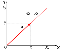

All non-zero vectors {$\mathbf{v}$} that satisfy such an equation are called eigenvectors of {$A$}, and their respective {$\lambda$} are called eigenvalues. “Eigen” is a German term, meaning “characteristic” or “peculiar to”, which is appropriate for eigenvectors and eigenvalues because to a great extent they describe the characteristics of the transformation that a matrix represents.

Now let’s go through a small example of how to find the eigenvalues and eigenvectors of a {$2 \times 2$} matrix by hand.

{$A = \left[ \begin{array}{cc} 2 & 1 \\ 1 & 2 \end{array} \right] \;\;\rightarrow\;\; \left[ \begin{array}{cc} 2 & 1 \\ 1 & 2 \end{array} \right] \left[ \begin{array}{cc} v_1 \\ v_2 \end{array} \right] = \lambda \left[ \begin{array}{cc} v_1 \\ v_2 \end{array} \right] \;\;\rightarrow\;\; \begin{array}{cc} 2v_1 + v_2 = \lambda v_1 \\ v_1 + 2v_2 = \lambda v_2 \end{array} \;\;\rightarrow\;\; \begin{array}{cc} (2 - \lambda)v_1 + v_2 = 0 \\ v_1 + (2 - \lambda)v_2 = 0 \end{array} \;\;\rightarrow\;\; (A - \lambda I)\mathbf{v} = 0$}

If {$(A - \lambda I)$} is invertible, then {$(A - \lambda I)^{-1} (A - \lambda I) \mathbf{v} = I \mathbf{v} = \mathbf{v} = 0$}, and thus the only solution to our system of equations would be the zero vector. Since an eigenvector by definition can’t be the zero vector, this is undesirable. To avoid choices of {$\lambda$} that make this system invertible, we can use our knowledge that a matrix is only invertible if it has a non-zero determinant. (Recall that the definition of the inverse of a matrix {$B$} includes the term {$1/|B|$}.) So, to find eigenvalues and eigenvectors, we require the determinant of {$(A - \lambda I)$} to be zero.

{$ | A - \lambda I | = \left| \begin{array}{cc} (2 - \lambda) & 1 \\ 1 & (2 - \lambda) \end{array} \right| = (2 - \lambda)(2 - \lambda) - 1*1 = \lambda^2 - 4 \lambda + 3 = (\lambda - 3)(\lambda - 1) = 0$}

To make the left hand side {$(\lambda - 3)(\lambda - 1)$} equal zero, we can either set {$\lambda = 3$} or {$\lambda = 1$}. Thus, these are the eigenvalues of {$A$}. To find the corresponding eigenvectors, we plug these values back into the original {$A\mathbf{v} = \lambda \mathbf{v}$} equations. We can determine the eigenvector using either of these two equations, so below we just show the derivation using {$2v_1 + v_2 = \lambda v_1$}.

{$ \; $ \begin{align*} &\lambda = 3:\; 2v_1 + v_2 = 3 v_1 \;\;\rightarrow\;\; v_1 = v_2 \\ &\lambda = 1:\; 2v_1 + v_2 = v_1 \;\;\rightarrow\;\; v_1 = -v_2 \\ \end{align*} $ \; $}

Any vector that satisfies either of these equations is an eigenvector of {$A$}. For example, the vectors {$\left[1, 1\right]^T$} and {$\left[1, -1\right]^T$} are eigenvectors of {$A$}. To summarize, the procedure for finding eigenvalues and eigenvectors for a matrix {$A$} is as follows:

• Set {$\det(A - \lambda I) = 0$} and solve for {$\lambda$}.
• Plug the resulting values back into the equations defined by {$A\mathbf{v} = \lambda \mathbf{v}$} and solve for {$\mathbf{v}$}.

Note that this is easy to do for a {$2 \times 2$} matrix because the characteristic polynomial is a quadratic. However, with larger matrices, the characteristic equation is a polynomial of higher degree. There is no closed-form expression (such as the quadratic formula) for finding the roots of polynomials of degree 5 or greater. There are iterative procedures for approximating these roots, but a problem they face is that the characteristic polynomial may be ill-conditioned. So, in practice, most eigenvalue solvers use alternative methods such as power iteration.

Why the Top k Eigenvectors of {$\Sigma$}

Now that we have some intuition for what eigenvalues and eigenvectors are, we can prove that the top k eigenvectors of the covariance matrix {$\Sigma$} are the directions along which our data {$D$} has the greatest variance. First, let’s try to find just one direction, the one along which our data has the most variance. Formally, our problem is to find the direction {$\mathbf{v}$} such that projecting our data {$X_c$} along it will maximize variance:

{$\max_{\mathbf{v}} E[(X_c\mathbf{v} - E[X_c\mathbf{v}])^2]$}

The above formula is just the definition of variance. (The notation {$X_c$} here is the same as that in the lecture notes; it refers to stacking the data into an n-by-m matrix, with the mean value of each feature subtracted out.) Let’s simplify this expression a little. Since {$\mathbf{v}$} is constant, we can pull it out of the internal expectation:

{$\max_{\mathbf{v}} E[(X_c\mathbf{v} - E[X_c]\mathbf{v})^2]$}

Then, because we normalized {$X_c$} so that every feature is zero-mean, we know {$E[X_c] = 0$}, so we can just remove it:

{$\max_{\mathbf{v}} E[(X_c\mathbf{v})^2]$}

Squaring and again moving {$\mathbf{v}$} outside the expectation we have:

{$\max_{\mathbf{v}} \mathbf{v}^T E[X^T_c X_c] \mathbf{v}$}

The expression {$E[X^T_c X_c]$} is exactly the covariance matrix. It is an {$m \times m$} matrix whose values are {$\Sigma = \frac{1}{n}\sum_{i=1}^n (\mathbf{x}^i-\mathbf{\overline x}) (\mathbf{x}^i-\mathbf{\overline x})^\top$}. (Try writing out the components of {$X^T_c X_c$} if this isn’t clear.) So, our maximization problem has been reduced to:

{$\max_{\mathbf{v}} \mathbf{v}^T \Sigma \mathbf{v}$}

Before completing the maximization, we have to add one constraint to the problem: {$\mathbf{v}^T\mathbf{v} = 1$}. This just requires that the vector representing the direction be of length 1. Otherwise we could infinitely increase the length of a vector to increase the value of the objective. We can add this constraint in using a Lagrange multiplier like so:

{$\max_{\mathbf{v}} \mathbf{v}^T \Sigma \mathbf{v} + \lambda (1 - \mathbf{v}^T\mathbf{v})$}

Taking the derivative with respect to {$\mathbf{v}$} and setting it equal to zero yields:

{$\Sigma \mathbf{v} - \lambda\mathbf{v} = 0$}

which means that the optimal {$\mathbf{v}$} is one such that {$\Sigma \mathbf{v} = \lambda\mathbf{v}$}. But this means {$\mathbf{v}$} exactly fits the definition of an eigenvector of {$\Sigma$}! So, clearly the {$\mathbf{v}$} we seek will be an eigenvector of {$\Sigma$}, but which eigenvector? Our overall problem is to maximize {$\mathbf{v}^T \Sigma \mathbf{v}$}, which we now know is equal to {$\lambda \mathbf{v}^T \mathbf{v}$}. Since we constrained {$\mathbf{v}$} to have length 1, {$\mathbf{v}^T \mathbf{v} = 1$}, and so what remains is just to maximize {$\lambda$}. We can do this by choosing the eigenvector with the largest eigenvalue. All this analysis can be repeated to find the second, third, fourth, etc. directions of greatest data variance, which will thus turn out to be the other top eigenvectors.

Singular Value Decomposition (SVD)

Computing the covariance matrix {$\Sigma$} and finding its eigenvectors is one way to do PCA. In the lecture notes you will find an alternative way though, which uses a technique called singular value decomposition (SVD):

PCA via SVD

• Given {$D = \mathbf{x}^1, \ldots, \mathbf{x}^n$}
• Compute {$\mathbf{\overline x} = \frac{1}{n}\sum_i\mathbf{x}^i$} and stack the data into n-by-m matrix {$X_c$} where where the rows are {$\mathbf{x}^i - \mathbf{\overline x}$}
• Compute SVD of {$X_c = U S V^\top$}
• Take k rows of {$V^\top$} with largest eigenvalues: {$\mathbf{v}_1,\ldots,\mathbf{v}_k$}, as principal components.
• Project: {$ \mathbf{z}^i = \left( (\mathbf{x}^i-\mathbf{\overline x})^\top\mathbf{v}_1, \ldots,(\mathbf{x}^i-\mathbf{\overline x})^\top\mathbf{v}_k \right)$}

Formally, the SVD of a matrix {$A$} is just the decomposition of {$A$} into three other matrices, which we’ll call {$U$}, {$S$}, and {$V$}. The dimensions of these matrices are given as subscripts in the formula below:

{$\textbf{SVD}:\;\;\; A_{n \times m} = U_{n \times n}S_{n \times m}V^T_{m \times m}.$}

The columns of {$U$} are orthonormal eigenvectors of {$AA^T$}. The columns of {$V$} are orthonormal eigenvectors of {$A^TA$}. The matrix {$S$} is diagonal, with the square roots of the eigenvalues from {$U$} (or {$V$}; the eigenvalues of {$A^TA$} are the same as those of {$AA^T$}) in descending order. These eigenvalues are called the singular values of {$A$}. For a proof that such a decomposition always exists, check out this SVD tutorial.

The key reason we would prefer to do PCA through SVD is that it is possible to compute the SVD of {$X_c$} without ever forming the matrix {$\Sigma$} matrix. Forming the {$\Sigma$} matrix and computing its eigenvalues using one of the methods suggested at the end of the eigen-things section above can lead to numerical instabilities. There are ways to compute the {$USV^T$} decomposition of SVD that have better numerical guarantees. (We won’t get into the particulars in this class though.)

SVD is a useful technique in many other settings also. For example, you might find it useful when working on the blog data for the project to try latent semantic indexing. This is a technique that computes the SVD of a matrix where each column represents a document and each row represents a particular word. After SVD, each column in the {$U$} matrix represents a general “concept”. For example, if our original set of words was [hospital nurse doctor notebook Batman], a column of {$U$} might have the entries {$\left[7, 10, 13, -22, -14\right]^T$}, indicating that hospital, nurse, and doctor all belong to one concept class, while notebook and Batman do not belong in this class.

Example of PCA for Faces

Suppose we had a set of face images (much like in the class project). We could use each pixel in an image as an individual feature. But this is a lot of features. Most likely we could get better performance on the test set using fewer, more generalizable features. PCA gives us a way to directly reduce and generalize the feature space. Here’s an example of how to do this in MATLAB: Eigenfaces.m.