Summary of the Class So Far
With {$n$} data points {$D = \{x_i, y_i\}$}, find a model that produces output {$y$} when given input {$x$}: {$h(x) = y$}. How do we find this model? Either we define a notion of error and try to minimize it, or we assume our data is drawn from a probability distribution and use it to define a data likelihood function which we try to maximize. To avoid overfitting, we either regularize by decreasing the number of parameters of our model so that it has lower variance, or we place a prior on the parameters, such as the Gaussian prior on each of the weights {$w_i$} in linear regression.
Single Sentence Lecture Summaries
- Point Estimation: Using data to compute a single “best” value for the parameters.
- Gaussians: Computing the parameters of a standard probability distribution.
- Regression: Can be thought of as just estimating another Gaussian (a conditional one).
- Bias Variance Decomposition: All models make tradeoffs between bias and variance; low bias allows for a better training data fit, low variance prevents overfitting, but you can only have both if the model is a good fit for the data.
- Classification: Instead of {$y \in \mathbb{R}$}, now {$y \in \{1, \ldots, K\}$}.
- Generative vs Discriminative: Discriminative models {$P(y|x)$}, while generative models {$P(x|y)P(y)$}.
- Naive Bayes: Generative classification model that makes the assumption all {$X_i$} are independent given {$Y$}.
- Logistic Regression: Discriminative classification model where each class is associated with a weight vector {$\mathbf{w_k}$}.
- Decision Trees: One popular method for building these is to use ID3’s “maximize information gain” heuristic.
- Cross-validation: Useful technique for preventing overfitting and for choosing how much influence to give to a regularization term.
- Boosting: Algorithm for turning a set of weak classifiers into a strong classifier, as well as “feature selection”.
- Nearest Neighbors: Predicts {$Y$}-value for a new point based on majority vote of its closest neighbors in {$X$}-space.
- Kernel Regression: Like nearest neighbors, but not all neighbors count equally: the vote of a neighbor is weighted by {$K(\textrm{neighbor's x value}, \textrm{test point's x value})$}, where {$K$} is some kernel.
- Locally Weighted Regression: Just like fitting a regular linear regression model, except that for each test point {$x$} we learn new parameters {$w(x)$} by weighing each train data points according to {$K(\textrm{train point's x value}, \textrm{test point's x value})$}.
- Kernel Methods: Writing linear and logistic regression in terms of weights on training examples {$\alpha$} instead of weights on features {$w$} allows us to refer to features only indirectly, through dot products. Then we can replace these dot products with any positive semi-definite function {$k$}, called a kernel.
3 views on learning algorithms
We can analyse how a learning algorithm works in three different spaces: the data view, the parameter view and the loss function view. It is a good exercise to find out, in each view, what makes each algorithm different from the others.
The data view
For any algorithm, we always start by describing what it does with the data:
- Continuous Y (regression) vs. discrete Y (classification)
- Continuous X vs. discrete X (type of probability modeling: Gaussian, Multinomial…)
- Local method (K-NN, kernel regression) vs. global method (LR, NB, DT, Boosting)
- Feature space (weight the features {$w^Tx$}) vs. dual space (weight the samples {$\alpha^Tk(x)$})
- Assumptions made by the classifier (is the NB assumption always justified? see homework question)
- …find more!
The parameter view
The parameter view is useful when an optimization is performed over the parameters (see practice exam question on optimization further down):
- MLE/MAP estimation: find the maximum of a log-concave function of the parameter
- Cross-validation: plot the error as a function of the parameter, and find the “magic” value
- More generally, we reason in the parameter space when adjusting the complexity of a model (bias-variance trade-off)
- Logistic regression: gradient ascent in the parameter space ({$w$})
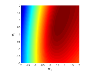 Log likelihood function heat map
The loss function view
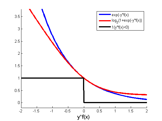
This view applies to classification tasks: for each example, how to penalize a misclassified example? We want {$y$} and {$f(x)$} to be of the same sign, so it makes sense to represent the loss as a function of {$yf(x)$}, which will be strictly negative if and only if {$x$} is misclassified:
- Where did these error functions come from?
(:answiki:)
- 1–0 loss function: It is the most classical error (used in cross-validation for instance): {$\varepsilon = \sum_i \mathbf{1}(y\ne f(x)) = \sum_i \mathbf{1}(yf(x)<0)$}
- Logistic regression loss: It comes from the cost function we optimize ({$\log(P(Y|X,w))$})
- Boosting (exponential loss): At each step {$t_0$}, the weights {$D_{t_0}(i)$} used in the error are exactly the exponential loss of the combined classifier so far.
(:answikiend:)
(:answiki:)
- Logistic regression: {$\max_w\log\left(\prod_i P(y_i|x_i,w)\right) = \min_w \sum_i \log (1+\exp(-y_i w^Tx_i))$}
- Boosting: At each step {$t_0$}, we optimize the weighted error on the {$N$} samples, and the weights are {$D_{t_0}(i) = \frac{1}{N}\frac{\exp(-y_if_{t_0}(x_i))}{\prod_{t=1}^{t_0} Z_t}$}
{$f_{t_0}(x)= \sum_{t=1}^{t_0} \alpha_t h_t(x)$} is the overall combined classifier so far (at {$t_0$}).
(We showed in the homework that {$\frac{1}{N}\sum_{i=1}^N\left(\exp(-y_if_{t_0}(x_i))\right) = \prod_{t=1}^{t_0} Z_t$}, which is another way of saying {$\sum_i D_{t_0}(i)=1$}).
(:answikiend:)
- What is the difference between logistic and exponential loss, the pros and cons of each?
(:answiki:)See the boosting lecture! To summarize:
- Logistic loss has a linear asymptote when {$yf(x)\rightarrow -\infty$}, so it is less harsh with misclassified points
- Exponential loss makes the boosting framework possible: as long as there is one weak classifier better than chance for the exponential error, the overall error keeps decreasing
(we established a bound on the error by leveraging the exponential loss in our derivation).
(:answikiend:)
Game: similarities and differences
Let’s take some concepts from the course and try to find what brings them together or breaks them apart:
(:answiki:)
- Similar: point estimation
- Different: MAP adds a prior
(:answikiend:)
- Logistic regression / Linear regression:
(:answiki:)
- Similar: regression! (LR solves classification as a regression problem)
- Different: for LR, the fitted function is not linear, it is the logistic function:
- Desired properties: we are fitting a probability, it has a value between 0 and 1 and p(-y|x,w) = 1 - p(y|x,w)
- Makes analogy to NB possible (same type of decision boundary)
- Saturation: misclassified examples that are far away from the boundary are not too penalized
(:answikiend:)
- Decision trees / Naive Bayes:
(:answiki:)
- Similar: Classification
- Different:
- Discriminative vs. generative
- NB assumption introduces a bias
- Decision trees have a higher risk of overfitting (pruning might be necessary)
- Training time and testing time
- NB: training is “fast” (estimate parameters by counting/averaging, scales with [number of parameters * size of data]), testing might be longer (evaluate {$P(Y=T,\mathbf{X})=P(Y=T)\prod_j P(x_j|Y=T)$}, scales with number of features)
- DT: training is long (ID3: try all splits, compute IG, repeat until leaf is reached), roughly scales with [2^(tree depth) * possible splits * tree width * size of data], testing is very fast (scales with tree depth, just one comparison at each level). This is why decision trees are popular to process Microsoft Kinect data in real-time.
(:answikiend:)
- Kernel regression from the first lecture / Kernel ridge regression in the kernel lecture
(:answiki:)
- Similar: The decisions are very similar, made by combining:
- the training labels {$y_1,\ldots,y_n$}
- the kernel products between train samples and the new test point {$k(x_1,x),\ldots,k(x_n,x)$}
- Different:
- In the first lecture, we used a Gaussian kernel {$k(x,x_i)=\exp\left(\frac{-\|x-x_i\|_2^2}{2\sigma^2}\right)$}.
- In the general kernel ridge regression we derived, {$k(x_1,x_2)$} can be anything, in particular it could be {$\Phi(x_1)^T\Phi(x_2)$} (see last week’s recitation)
- Similarity of the output {$\hat{y}$}
- Kernel regression (KR): {$\hat{y}(x)=\frac{\sum_i k(x,x_i)y_i}{\sum_i k(x,x_i)} = \frac{\mathbf{k(x)}^T\mathbf{y}}{\mathbf{k(x)}^T\mathbf{1}}$}
- Kernel ridge regression (KRR): {$\hat{y}(x)=\mathbf{x}^TX^T\mathbf{\alpha} = (X\mathbf{x})^T\mathbf{\alpha} = \mathbf{k(x)}^T\mathbf{\alpha}$}
where {$\mathbf{\alpha} = (K+\frac{\sigma^2}{\lambda^2}I)^{-1}\mathbf{y}$}
- Conclusion: just as in KR, the {$\alpha_i$}’s of KRR contain the {$y_i$}’s but also include a regularization term.
(:answikiend:)
- Exercise: practice making other comparisons
Short review of kernel methods
- Starting point: classification/regression with a linear boundary (output of form {$f(w^Tx)$}: linear/logistic regression) and regularization.
Here let’s say X is an N-by-d matrix
- Notice that optimal {$w_{MAP}$} can be written as {$X^T\alpha_{MAP}$} (combination of the samples)
- Therefore let’s express any candidate {$w$} as {$X^T\alpha$}
- Now we’re optimizing over {$\alpha$} instead of {$w$}.
- Why do we do this change of variable?
(:answiki:)
- X disappears too!
- {$Xw = X\mathbf{(X^T\alpha)} = \mathbf{K}\alpha$}
- {$x^Tw = x^T\mathbf{(X^T\alpha)} = (Xx)^T \alpha = \mathbf{k(x)}^T \alpha$}
- We don’t need the features anymore, everything is in terms of {$\alpha$}, {$k(x)$}, and/or {$K$}
- {$K = XX^T$} is the N-by-N Gram matrix
({$K_{i,j} = k(x_i,x_j)$})
- {$k(x) = Xx$} is the N-by-1 vector of inner products with {$x$}
({$k(x)_i = k(x_i,x)$})
(:answikiend:)
To summarize: {$w^Tx \leftrightarrow \alpha^Tk(x)$}
- Note that {$w$} and {$x$} are of size d, and {$\alpha$} and {$k(x)$} are of size N
- Understand where it comes from and why it’s cool.
(:answiki:)
- We are reasoning in terms of similarities with other samples instead of features
- The computation of {$K$} and {$k(x)$} scales with dataset size and similarity function k (could be anything)
- The feature space (where {$x$} lies) could be of huge dimension but as long as evaluating k is fast, that’s ok!
(:answikiend:)
(:answiki:)
- Combine a large number of features (more information) but keep decision fast by using a fast similarity (kernel) function
- Express {$k(x_1,x_2)=\mathbf{\Phi}(x_1)^T\mathbf{\Phi}(x_2)$}: lift the features ({$x\rightarrow \Phi(x)$}) to learn a non-linear boundary
(:answikiend:)
- What does it change in practice?
| Algorithm | Ridge regression | Kernel ridge regression |
|---|
| Training | Find optimal {$w_{MAP}$} (closed-form as a function of {$X$},{$\lambda$},{$\sigma$}) | Precompute K, find optimal {$\alpha_{MAP}$} (closed-form as a function of {$K$},{$\lambda$},{$\sigma$}) |
|---|
| Testing | For given x, return {$w_{MAP}^Tx$} | Compute k(x), return {$\alpha_{MAP}^Tk(x)$} |
|---|
Practice Problems
You can find some additional good practice problems in these past exams from a CMU course. Not all the questions are relevant to the material we’ve covered, but given the large number of past exams there, you should still be able to find many problems that are relevant.
Shorts
- True or False: A classifier trained on less training data is less likely to overfit. (:ans:)
False. A specific classifier (with some fixed model complexity) will be more likely to fit to the noise in the training data when there is less training data, and is therefore more likely to overfit.
(:ansend:)
- In logistic regression, you observe that your gradient descent algorithm seems to never converge; the cost function (-log likelihood) keeps decreasing, and the weights learned approach infinity. What is going on? What is one way to prevent this? (:ans:)
The data is perfectly separable, so the likelihood can approach 1, and the sigmoid can approach a step function as the weights approach infinity. To see why the weights can approach infinity, consider binary logistic regression, and recall that at the decision boundary {$P(Y = -1 \mid \textbf{x}) = P(Y = 1 \mid \textbf{x})$}, which implies the form of the boundary is {$\textbf{w}^T \textbf{x} = 0$}. Writing this in standard slope-intercept form:
{$x_1 = \frac{w_2 x_2 + w_3 x_3 + \ldots}{w_1} + \frac{w_0}{w_1} $}
From this, it is clear that we can increase the magnitude of the {$w_i$} infinitely, and the decision boundary won’t change as long as the ratios {$\frac{w_2}{w_1}$}, {$\frac{w_3}{w_1}$}, etc. don’t change.
To fix this problem of infinite weights, use regularization (Gaussian zero-mean prior on each weight).
(:ansend:)
- For kernel regression, which of these structural assumptions is the one that most affects the trade-off between overfitting and underfitting:(:ans:)
(c) The kernel width. Small kernel width means only training points very close to a test point will influence the prediction for that test point. This can result in overfitting. On the other hand, if kernel width is too large, this can result in underfitting.
(:ansend:)
- (a) Whether kernel function is Gaussian versus triangular versus box-shaped
- (b) The kernel width
- (c) Whether we use Euclidean versus {$L_1$} versus {$L_\infty$} metrics
- (d) The maximum height of the kernel function
- Which of the following is Bayes rule?(:ans:)
(c) {$P(X \mid Y) = \frac{P(Y \mid X) P(X)}{P(Y)}$}. This follows directly from the definition of conditional probability:
{$ \; $ \begin{align*} P(X \mid Y) &= \frac{P(X, Y)}{P(Y)} \\ P(Y \mid X) &= \frac{P(X, Y)}{P(X)} \\ \end{align*} $ \; $}
Isolating the {$P(X,Y)$} term on the right side of each of these equations, then setting them equal, we arrive at Bayes rule.
(:ansend:)
- (a) {$P(X_1, X_2 \mid Y) = P(X_1 \mid Y) P(X_2 \mid Y)$}
- (b) {$P(Y \mid X_1, X_2) = P(Y \mid X_1) P(Y \mid X_2)$}
- (c) {$P(X \mid Y) = \frac{P(Y \mid X) P(X)}{P(Y)}$}
- (d) {$P(X \mid Y) = \frac{P(Y \mid X) P(Y)}{P(X)}$}
- Suppose you know {$X_1$} and {$X_2$} are independent random variables, and you want to use them to predict {$Y$}. Is it possible that Naive Bayes might be outperformed by any other classifier (e.g., decision tree, logistic regression)? (:ans:)
Yes, another method might outperform Naive Bayes, because the independence assumptions it makes might not be true in this case. Although {$X_1$} and {$X_2$} are independent, they are not necessarily independent given {$Y$}, which is the assumption the Naive Bayes likelihood makes: {$P(Y \mid X_1, X_2) = P(Y) P(X_1 \mid Y) P(X_2 \mid Y)$}. Take the XOR function for example. In that case, {$X_1$} and {$X_2$} are independent, but {$Y = X_1 \;\;\textrm{XOR}\;\; X_2$}, so {$P(X_1, X_2 \mid Y) \neq P(X_1 \mid Y) P(X_2 \mid Y)$}.
(:ansend:)
- If you run Adaboost with multinomial Naive Bayes as the weak classifier, how many parameters will you be storing after {$T$} iterations of boosting? Consider the case where the multinomial Naive Bayes classifier has a single output value {$Y$} that can be in any of {$K$} classes {$\{1, \ldots, K\}$}, and {$M$} input features {$X_1, \ldots X_M$} that can each take on {$L$} values {$\{1, \ldots, L\}$}. (:ans:)
Each iteration of boosting will add one multinomial Naive Bayes classifier that you must store, plus an {$\alpha_t$} value to weight the vote of this classifier. A single multinomial Naive Bayes classifier requires {$K - 1$} parameters for {$P(Y = 1), \ldots, P(Y = K - 1)$}. It also requires {$P(X_i = 1 | Y = j), \ldots, P(X_i = L - 1 | Y = j)$} for all {$j \in \{1, \ldots, K\}$} and all {$i \in \{1, \ldots, M\}$}, a total of {$(L - 1)KM$} parameters. Overall, that’s {$(K - 1) + (L - 1)KM$} parameters for a single multinomial Naive Bayes classifier. Adding {$T$} parameters for the {$\alpha_t$}, the total parameter storage count is {$T + T*[(K - 1) + (L - 1)KM]$}.
(:ansend:)
Optimal ML
Many machine learning algorithms can be formulated as solving an optimization problem. For some of them, optimal solutions are guaranteed, but sadly, not always. For each machine learning algorithm below, choose true (T) or false {$('''F''')$} with respect to the following statement: The algorithm always reaches an optimal solution.
- {$\textbf{T/F}$}: linear regression (:ans:) True. There is a closed-form solution for the optimal weights: {$\textbf{w} = (X^T X)^{-1}X^T \textbf{y}$}. (:ansend:)
- {$\textbf{T/F}$}: linear regression with {$L_2$} regularization: {$\lambda ||w||_2^2$} (:ans:) True. Again, there is a closed-form solution for the optimal weights: {$\textbf{w} = (X^T X + \frac{\sigma^2}{\lambda^2}I)^{-1}X^T \textbf{y}$}. (:ansend:)
- {$\textbf{T/F}$}: logistic regression (:ans:) True. Using gradient ascent on the likelihood, {$\textbf{w}_{t + 1} = \textbf{w}_t + \eta \nabla_{\textbf{w}}\ell(\textbf{w})$}, we eventually converge to the optimal {$\textbf{w}$} (as long as the learning rate {$\eta$} is small enough), since the likelihood is a concave function. (:ansend:)
- {$\textbf{T/F}$}: learning decision trees with the ID3 algorithm (:ans:) False. The tree is grown greedily with only 1-step look-ahead. Thus, though the resulting tree may be consistent on the train set (0 train error), it will still likely be suboptimal in the sense that there will likely exist a consistent tree of smaller depth. (:ansend:)
- {$\textbf{T/F}$}: Gaussian or Multinomial point estimation (:ans:) True. Indeed these estimations can be seen as optimizations over the parameter. There is a guaranteed optimum because the likelihood (and prior for MAP) are log-concave functions of the parameters. Again, there are closed-form solutions. (:ansend:)