ClassificationOn this page… (hide) 1. Classification ReviewWe’re going to be talking about binary classification: as you may remember, the goal here is to predict a label {$y$} from input examples {$\mathbf{x}$}, where {$y$} can take on one of two values, typically either {$-1$} or {$+1$}. 2. Gaussian Naive Bayes (GNB) vs. Logistic RegressionThere’s many ways we could attempt to solve this problem, but we’re going to focus on two that we’ve covered in class recently: Gaussian Naive Bayes and Logistic Regression. How do these methods work? At a high level, we:
{$h(\mathbf{x}) = \arg \max_y \hat{P}(y\mid\mathbf{x}).$} As covered earlier, one difference between GNB and logistic regression is how the distribution {$\hat{P}(y\mid \mathbf{x})$} is estimated: {$ \textrm{GNB: } \hat{P}(y \mid \mathbf{x}) \propto \underbrace{P(y)}_{\rm class prior} \underbrace{P(\mathbf{x}\mid y)}_{\rm class model}, \qquad \textrm{LR: } \hat{P}(y \mid \mathbf{x}) = \frac{1}{1+ \exp\{-y\mathbf{w}^\top\mathbf{x}\}} $} We’re now going to take a more detailed, nuanced view at the consequences of these two different means of achieving the same goal. In other words, we’re going to ask the question, how and why will LR and GNB come up with two different answers for the same problem? 2.1 GNB with shared variances vs. LRTo start with we’ll look at a specific variant of GNB. Let’s look at the analysis at the end of the lecture on logistic regression. At a high level, the result is as follows: for a specific variant of GNB where the variance parameter is shared among classes, the decision rule for GNB is of the same parametric form as logistic regression. Question: What can we say about the decision boundary for GNB with shared variances? Since the decision boundary has the same parametric form as that for logistic regression, it will also be a linear decision boundary. Question: Does this mean that GNB with shared variances and logistic regression will find the same decision boundary on a given problem? No. Remember that the fitting process for GNB is different than that for logistic regression. For logistic regression, we maximize the conditional likelihood of the labels given the data: (:centereq:) {$\log P(\mathbf{Y}\mid\mathbf{X}) = \sum_i \log P(y_i \mid \mathbf{x}_i)$} (:centereqend:) For GNB, we maximize the joint likelihood of the labels and the data: (:centereq:) {$\log P(\mathbf{Y}, \mathbf{X}) = \sum_i \log P(y_i,\mathbf{x}_i) = \sum_i \log P(y_i) + \log P(\mathbf{x}_i \mid y_i)$} (:centereqend:) These two different objective functions will lead to different methods of fitting (gradient descent for LR, and an analytic solution for GNB) that may lead to two different decision boundaries. 2.2 When data is linearly separableNow we will examine a situation where the differences between GNB and LR can lead to different behavior during the training process. Suppose we are given a dataset like this: 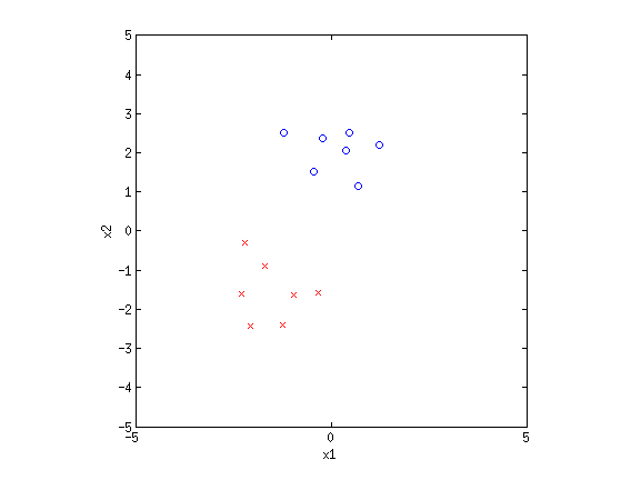 Clearly this dataset is linearly separable: we can separate the 2 classes perfectly by drawing a line between them in the space of {$\mathbf{x}$}. Now, suppose I tell you that the parameters {$\mathbf{w} = [-1.5, 3]$} separates the data perfectly. Then so does {$\mathbf{w} = [-3, 6]$}, {$\mathbf{w} = [-6, 12]$}, and so on: any {$\mathbf{w}' = \alpha\mathbf{w}$} will also result in a perfectly separating hyperplane. Let’s see what happens to the log conditional likelihood as {$\alpha \rightarrow \infty$}: {$ \log P(\mathbf{Y}\mid\mathbf{X}) = -\sum_{i} \log (1+\exp\{-\alpha y_i\textbf{w}^\top\textbf{x}_i\}) $} However, we know that {$\mathbf{w}$} separates the data perfectly: this means that {$\mathrm{sign}\left(\mathbf{w}^\top\mathbf{x}_i\right) = y_i$}, so {$y_i\textbf{w}^\top\textbf{x}_i$} is just some constant value {$c_i$} where {$c_i > 0$}. So we have: {$ \log P(\mathbf{Y}\mid\mathbf{X}) = -\sum_{i} \log (1+\exp\{-\alpha c_i\})$} Clearly, as {$\alpha \rightarrow \infty$}, {$\exp\{-\alpha c_i\} \rightarrow 0$}, so {$\log P(\mathbf{Y}\mid\mathbf{X}) \rightarrow 0 \quad \textrm{as} \quad \alpha \rightarrow \infty.$} Question: Since {$\log P = 0$} implies {$P = 1$}, what does the above result imply about “cranking up” a weight vector {$\mathbf{w}$} that perfectly separates the data? What does the above result imply about our gradient descent fitting algorithm? If we have {$\mathbf{w}$} that perfectly separates the data, we can increase the conditional likelihood of the data simply by scaling the vector higher and higher. In other words, the gradient will always “point” in the direction of increasing {$||\mathbf{w}||$}: if we allowed gradient descent to run forever, it would never converge. Question:Does any of the above analysis change if use MAP estimation and apply a zero-mean Gaussian prior to {$\mathbf{w}$}? Yes! Remember that the effect of the prior is to penalize large values of {$||\mathbf{w}||$}. The argument above states that increasing {$||\mathbf{w}||$} increases the conditional likelihood of the data, but if we apply a prior, we will simultaneously increase the conditional likelihood of the data and decrease the prior probability of the parameters {$\mathbf{w}$}. Eventually, these two forces will balance each other, and increasing {$||\mathbf{w}||$} will no longer increase the posterior probability of {$||\mathbf{w}||$} given the data. Therefore our MAP estimation gradient descent algorithm will eventually converge. This was just one example of how an infinite number of linear separating hyperplanes can get us into trouble with algorithms that don’t have any means of distinguishing between two “perfect” solutions {$\mathbf{w}$} and {$\mathbf{w}'$}. Perfectly separable data is actually quite common in some application areas. For instance, in any field where obtaining measurements is hard but many measurements can be obtained in parallel, it is often the case that the number features far exceeds the number of examples. For instance, a functional Magnetic Resonance Imaging (fMRI) scan provides measurements of brain activity at 80,000 locations simultaneously across the brain, but we can only typically take ~100 measurements in a given scanning session. Mathematically, if we are looking for a linear prediction, {$\mathbf{y} = \mathbf{X}\mathbf{w},$} but the number of rows of {$\mathbf{X}$} exceeds the numbers of columns of {$\mathbf{X}$}, we can almost always find a solution {$\mathbf{w}^\star$} such that {$\mathbf{X}\mathbf{w}^\star = \mathbf{y}$}, regardless of the values of {$y$}. Question: Does GNB suffer from the same problem? No. As we’ve seen, the parameters for GNB have an analytic solution: the mean and variances of the points within the different classes. Linear separation doesn’t come into the picture. 2.3 Naive Bayes vs Logistic Regression in generalA well-known paper of Andrew Ng and Michael Jordan finds mathematical and experimental foundations for the following: As the number of training samples {$n$} goes to infinity, very often, logistic regression has a lower asymptotic error than does naive Bayes. However, naive Bayes converges more quickly to its (higher) asymptotic error. Thus, very often, as the number of training samples is increased, naive Bayes initially performs better but is then overtaken by logistic regression. 3. Basis functionsEven though LR and sometimes GNB result in linear decision boundaries, we can still potentially learn very difficult, non-separable datasets by transforming the inputs using basis functions. For example, consider the XOR dataset: 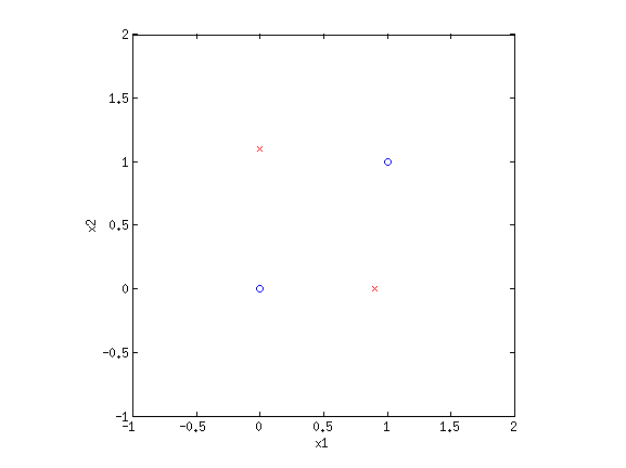 Clearly this is not separable. But by transforming the input into a new space, this dataset can be made separable. Consider {$\phi_1(\mathbf{x}) = x_1+x_2$} and {$\phi_2(\mathbf{x}) = x_1\cdot x_2$}. If we plot the same data along the new dimensions {$\phi_1$} and {$\phi_2$}, we find: 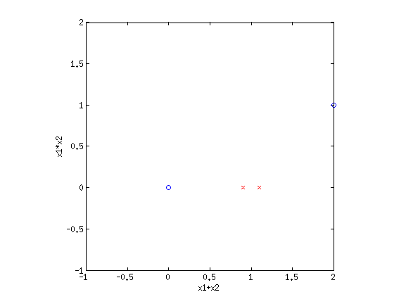 The data is now separable! Let’s look at another example. 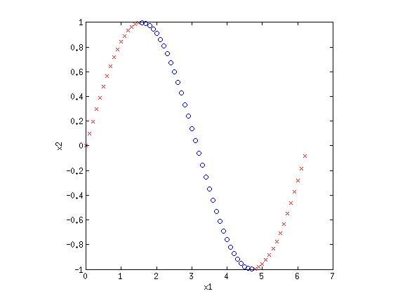 This looks like a sin function, and it is also not separable. However, if we could “flip” the orientation of the curve, we could draw a line through the data. Let’s consider the new basis {$\phi_1(\mathbf{x}) = x_1$} and {$\phi_2(\mathbf{x}) = \cos x_1$}: 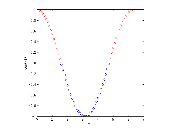 Now we have once again transformed a non-linearly separable dataset into one that is linearly separable. 3.1 Practice problemsWhat basis functions could we use to make the following datasets linearly separable? 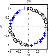
One way to transform this is to notice that the quadrants where {$\mathrm{sign}\left(x_1\right) = \mathrm{sign}\left(x_2\right)$} are the same class. Therefore we could use a single basis function {$\phi(\mathbf{w}) = x_1 \cdot x_2$}, and would separate this data along a single line. 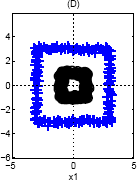
Again, we can use a single basis function: {$\phi(\mathbf{x}) = ||\mathbf{x}||_2$}, since the inner class is closer to the center (and therefore smaller norm) than the outer class. 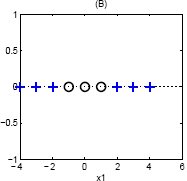
Consider the basis, {$\phi_1(\mathbf{x}) = x_1, \phi_2(\mathbf{x}) = x_1^2$}. This will raise the line into a parabola, with the top of the parabola being separable from the bottom half. These are all carefully constructed toy examples, but the point is to demonstrate that determining what is linearly separable is not an easy question. As the saying goes, one man’s garbage is another man’s linearly separable dataset. |