|
Lectures /
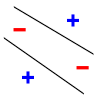
VC DimOn this page… (hide) Generalization bounds for infinite classes: VC dimensionWe will now consider the case where our hypothesis space is infinite, for example, hyperplanes of dimension {$m$}. As before, our learning algorithm selects a hypothesis h from {$\mathcal{H}$} based on a sample {$D$} of n i.i.d. examples {$\{\mathbf{x}_i,y_i\}$} from {$P(\mathbf{x},y)$}, which will denote as {$D\sim P^n$}. We will denote the {$0/1$} training data error (also called loss) of a hypothesis h as {$L_D(h) = \frac{1}{n} \sum_i \mathbf{1}(h(\mathbf{x}_i)\ne y_i)$} and we’ll denote the true error as {$L_P(h) = \mathbf{E}_{(\mathbf{x},y)\sim P} [\mathbf{1}(h(\mathbf{x})\ne y)]$} For finite hypothesis spaces, we showed in the last lecture that: Theorem: With probability {$1-\delta$} over the choice of training sample of size {$n$}, for all hypotheses {$h$} in {$\mathcal{H}$}: {$L_P(h) - L_D(h) \le \sqrt{\frac{\log |\mathcal{H}| + \log\frac{1}{\delta}}{2n}}$} We now consider the case of infinite hypothesis spaces, for example, hyperplanes. To bound the error of a classifier from a class {$\mathcal{H}$} using {$n$} examples, what matters is not the pure size of {$\mathcal{H}$}, but its richness: the ability to fit any dataset of size {$n$} perfectly. Perhaps the most fundamental measure of richness (or power or complexity or variance) of a hypothesis class studied in machine learning is called the Vapnik-Chervonenkis dimension (named for two Russian mathematicians, Vladimir Vapnik and Alexey Chervonenkis). For example, one can show that the VC-dimension of a class of hyperplanes of dimension {$m$} is {$m+1$}. In general, VC-dimension can be related to the number of parameters in a very complicated way. A fundamental result by Vapnik and Chervonenkis is that the {$\log |\mathcal{H}|$} in the bounds can be replaced by a function of the {$VC(\mathcal{H})$}: Theorem: With probability {$1-\delta$} over the choice of training sample of size {$n$}, for all hypotheses in {$\mathcal{H}$}: {$L_P(h) - L_D(h) \le \sqrt{\frac{VC(\mathcal{H})(\log\frac{2n}{VC(\mathcal{H})} + 1) + \log\frac{4}{\delta}}{n}}$} We will not prove this theorem, as the proof is somewhat involved. In order to understand what it means, we need to define several terms. VC-dimension of hyperplanesConsider linear separators in 2 dimensions: {$sign(w_1 x_1 + w_2 x_2 + b)$}. For a set of three non-collinear points, there are {$2^3 =8$} possible labelings, and we can always find a hyperplane with zero error:
However, with 4 points, there are labelings no hyperplane in 2D can fit: 
More generally, we define the notion of shattering. Definition: A hypothesis class {$\mathcal{H}$} shatters a set of instances {$S = \{\mathbf{x}_1,\ldots,\mathbf{x}_n\}$} where {$\mathbf{x}_i \in \mathcal{X}$} if for every possible labeling {$\{y_1,\ldots,y_n\}$} with {$y_i\in\pm 1$}, there is an {$h\in\mathcal{H}$} with zero error: {$h(\mathbf{x}_i) = y_i, \;\; i=1,\ldots,n$}. So hyperplanes in 2-D shatter any set of 3 non-collinear points, but there are sets of 4 points in 2-D that cannot be shattered by 2D hyperplanes. VC-dimension measures the size of the largest set that can be shattered by the class. Definition: The VC-dimension of a class {$\mathcal{H}$} over the input space {$\mathcal{X}$} is the size of the largest finite set {$S \subset \mathcal{X}$} shattered by {$\mathcal{H}$}. To show the VC-dimension of a class is v, we need to show:
Proof sketch of {$VC(\mathcal{H}) = 3$} for 2D hyperplanes {$\mathcal{H} = \{ h(\mathbf{x}) = sign(w_1 x_1 + w_2 x_2 + b)\}$}.
In general, we can show the VC dimension of hyperplanes in m dimensions is {$m+1$}. However, the number of parameters of a classifier is not necessarily it’s VC dimension. Here are few other examples. Classes with infinite VC dimension
|