|
Lectures /
Point EstimationOn this page… (hide) Point Estimation Basics: Biased CoinBefore we get to any complex learning algorithms, let’s begin with the most basic learning problem.  A biased coin
Suppose you found a funny looking coin on your way to class and, being a scientist, started flipping it.
What is the simplest model of this scientific experiment? Each flip is a Bernoulli (binary) variable, independently and identically distributed (i.i.d.): {$P(H) = \theta \; {\rm and} \;P(T) = 1-\theta, \; {\rm where}\; \theta \in [0,1].$} So if you flip the coin {$n$} times, with {$n_H$} heads and {$n_T$} tails, the likelihood of observing a sequence (data) D is: {$ P(D\mid\theta) = \theta^{n_H}(1-\theta)^{n_T}$}. Maximum Likelihood Estimation (MLE) for the coinSuppose you observe 3 heads and 2 tails. What’s your guess for {$\theta$}? If you guessed 3/5, you might be doing MLE, which is simply finding a model that best explains your experiment: {$ \hat\theta_{MLE} = \arg \max_\theta P(D\mid\theta)$} How do we find the {$\theta$} that maximizes the log-likelihood of the data? Let’s try to take the derivative and set it equal to zero. Before we do that though, let’s change the product of {$\theta$}-dependent terms to a sum of terms --- this will make it slightly easier to deal with the derivative. We can get a sum from our product by simply taking the log: {$\log P(D\mid\theta) = n_H\log(\theta) + n_T\log(1-\theta)$} Notice that since log is a an increasing monotonic function, taking the log doesn’t change the {$\arg \max$}: {$\arg \max_\theta P(D\mid\theta) = \arg \max_\theta \; \log P(D\mid\theta)$} so taking log in this case doesn’t change the overall answer we’ll get for {$\theta$}. Now, let’s take the derivative and set it equal to zero: {$ \; \begin{align*} \frac{d}{d\theta} \log P(D\mid\theta) & = 0 \\ \frac{n_H}{\theta} - \frac{n_T}{1 - \theta} & = 0 \\ n_H(1 - \theta) & = n_T\theta \\ \hat\theta_{MLE} & = \frac{n_H}{n_H+n_T}. \end{align*} \; $} Why and when is it a good idea to set the parameters of a model by MLE? In practice, the MLE principle is a basis for a majority of practical parameter estimation algorithms, as we will see. If you have enough data and the correct model, MLE is all you need: it will find the true parameters. The problem is that you rarely have either enough data or the perfect model, so MLE can be terribly wrong. Example: suppose all five tosses come up heads, would you believe MLE? What about five million tosses, all heads? As another example, consider deriving MLE for the multinomial distribution for estimating a model of a die (ours is a different definition than wikipedia). Suppose there are {$K$} sides of the die (let’s call them labels or outcomes), so the model is {$P(X = j) = \theta_j \;\; 1 \le j \le K-1, \; \; P(X = K) = 1 - \sum_{j=1}^{K-1} \theta_j $} (We can also define {$\theta_K$} and introduce a sum to 1 constraint on the parameters — then we would have to use the method of Lagrange multipliers — we’ll do it that way later in the course: https://alliance.seas.upenn.edu/~cis520/wiki/index.php?n=Lectures.EM, see M-step…) We are given a dataset D of {$n$} samples, of which {$n_j$} have label/outcome {$j$} and {$n = \sum_{j=1}^K n_j$}. The log likelihood is {$\log P(D|\theta) = \sum_{j=1}^{K-1} n_j \log \theta_j + n_K \log (1 - \sum_{k=1}^{K-1} \theta_k ) $} Taking partial derivates for each parameter, we have: {$ \begin{align*} \frac{\partial}{\partial\theta_j} \log P(D\mid\theta) & = 0, \;\;\; 1 \le j \le K-1 \\ \frac{n_j}{\theta_j} - \frac{n_K}{1 - \sum_{k=1}^{K-1}\theta_k} & = 0, \;\;\; 1 \le j \le K-1\\ \frac{1-\sum_{k=1}^{K-1} \theta_k }{n_K} &= \frac{\theta_j}{n_j}, \;\;\; 1 \le j \le K-1 . \end{align*} $} Since the last equation holds for every j and the left hand side does not depend on j, we have that for some constant C, {$ \theta_j = C n_j, \;\; 1 \le j \le K-1,\;\; {\rm and} \;\; 1-\sum_{k=1}^{K-1} \theta_k = C n_K $}. Plugging in {$ \theta_j = C n_j $} into the last equation, we have: {$ 1-\sum_{k=1}^{K-1} C n_k = C n_K $}. So C is 1/n. Hence the MLE is {$ \theta_j =\frac{n_j}{n} , \;\; 1 \le j \le K-1 $}. Learning guaranteesHow sure can you be in your estimate, supposing you still believe your model? The following bound (based on the Hoeffding inequality) will be very useful later in the course: {$P(|\hat\theta_{MLE} - \theta^*| \ge \epsilon)\le 2e^{-2n\epsilon^2,}$} where {$\theta^*$} is the true parameter and {$\epsilon > 0$}. In words: The probability of the observed proportion of heads deviating by {$\epsilon$} from the true proportion in an i.i.d. sample of n tosses decreases exponentially with n and {$\epsilon$}. So, how much data do I need if I want to be 95% sure that I guessed the proportion plus/minus 0.1? We can solve for n as follows: {$ \; \begin{align*} P(|\hat\theta_{MLE} - \theta^*| \ge \epsilon) & \le (1 - 0.95) \\ \rightarrow 1 - 0.95 & = 2e^{-2n*0.1^2} \\ n & = \frac{\log \frac{2}{0.05}}{2*0.1^2}\approx 185. \end{align*} \; $} Here and below, log is the natural log. In general, if I want {$1-\delta$} confidence with {$\epsilon$} (absolute) error, I need: {$n \ge \frac{\log \frac{2}{\delta}}{2\epsilon^2}.$} Here are the required number of independent tosses for several values of confidence {$\delta$}: 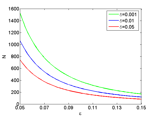 A plot of the bound for several values of delta
Guarantees of this kind are what the Probably Approximately Correct (PAC) framework aims to derive for learning algorithms, where the key goal is polynomial or better dependence of n (sample complexity) on other factors. We’ll talk about this much more later in the course. The Bayesian wayThe fact is, that you have some experience with coins, so when you don’t have enough data, you rely on your prior knowledge that most coins are pretty fair to estimate the parameter. If you’re a Bayesian, you will embrace uncertainty but quantify it, by assuming that your prior belief about coin fairness can be described with a distribution {$P(\theta)$}. In particular, the Beta distribution, with several examples shown below, is a very convenient class of priors: 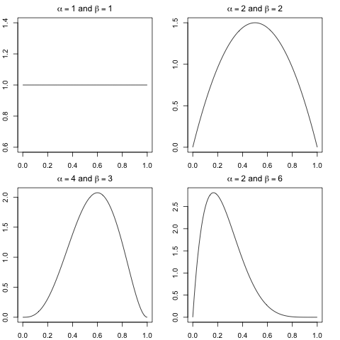 We’ll talk about the exact form of the prior in a moment, but first, what do we do with it? The Bayesian framework uses data to update this prior distribution over the parameters. Using Bayes rule, we obtain a posterior over parameters: {$ P(\theta | D) = \frac{P(D | \theta) P(\theta)}{P(D)} \propto P(D | \theta) P(\theta) $} Now let’s look at the Beta distribution: {$ Beta(\alpha,\beta):\;\; P(\theta \mid \alpha,\beta) = \frac{\Gamma(\alpha+\beta)}{\Gamma(\alpha)\Gamma(\beta)}\theta^{\alpha-1}(1-\theta)^{\beta-1}$} where {$\Gamma$} is the gamma function (for positive integers n, {$\Gamma(n)=(n-1)!$}). The hyperparameters {$\alpha\ge 1,\beta \ge 1 $} control the shape of the prior: their sum controls peakiness and their ratio controls the left-right bias. Why is Beta so convenient? Here’s why: {$ P(\theta | D) \propto P(D | \theta) P(\theta) \propto \theta^{n_H+\alpha-1}(1-\theta)^{n_T+\beta-1}$} Hence, {$ P(\theta | D) = Beta(n_H+\alpha;n_T+\beta)$}. This property of fit between a model and its prior is called conjugacy, which essentially means the posterior is of the same distributional family as the prior. OK, so now we have a posterior, but what if we want a single number (an estimate). The most common answer, basically because it is often computationally the easiest, is the maximum a posteriori (MAP) estimate: {$ \hat\theta_{MAP} = \arg \max_\theta P(\theta\mid D) = \arg \max_\theta \left( \log P(D\mid\theta) + \log P(\theta) \right)$} For the {$ Beta(\alpha;\beta)$} prior, the MAP estimate is: {$ \hat\theta_{MAP} = \frac{n_H+\alpha-1}{n_H+n_T+\alpha+\beta-2} $} Note that as {$ n = n_H+n_T \rightarrow \infty$}, the prior’s effect vanishes and we recover MLE, which is what we want: in the evidence of enough data, prior shouldn’t matter. We will see this vanishing prior effect in many scenarios. MAP estimate is only the simplest Bayesian approach to parameter estimation. It sets our model parameter to the mode of the posterior distribution {$ P(\theta\mid D) $}. There is much more information in the posterior than is expressed by the mode; for instance, the posterior mean and variance of the parameter. Why the mean? Suppose you want to predict what the probability of the next flip coming up heads is, given the seen data is exactly the posterior mean: {$ \; \begin{align*} P(X_{n+1} = H \mid D) & = \int_\theta P(X_{n+1}= H,\theta\mid D)d\theta \\ & = \int_\theta P(X_{n+1} = H \mid \theta)P(\theta\mid D)d\theta \\ & = \int_\theta \theta P(\theta\mid D)d\theta \end{align*} \; $} |