|
Lectures /
Matrices And TensorsLinear Algebra ReviewVector BasicsFor {$m$}-dimensional vectors {$\mathbf{v}$} and {$\mathbf{u}$} that form angle {$\theta$} with each other:
Vectors of unit length ({$|\mathbf{v}| = 1$}) are called normal vectors. Two vectors {$\mathbf{v}$} and {$\mathbf{u}$} are said to be orthogonal, {$\mathbf{v} \perp \mathbf{u}$}, if {$\mathbf{v} \cdot \mathbf{u} = 0$}. In {$2D$} this corresponds to them being at a {$90^\circ$} angle. Two normal vectors that are orthogonal are called orthonormal. You can get a geometric intuition for the dot product and orthogonality by playing with this dot product applet. Note that for the purposes of multiplication, it’s convention to assume vectors are vertical, and that their transposes are horizontal as shown below. {$\mathbf{v} = \left[\begin{array}{c} v_1 \\ \vdots \\ v_m \end{array}\right] \;\;\;\;\;\;\textrm{and}\;\;\;\;\;\; \mathbf{v}^T = \left[\begin{array}{ccc} v_1 & \ldots & v_m \\ \end{array}\right]$} Geometrically, a vector can be viewed as a point in a space. Multiplying by a scalar lengthens (or shortens) the vector, changing its norm (length). A vector can also be thought of as a mapping (using a dot product) from a vector to a scalar. Matrix BasicsAn {$n*m$} matrix {$\mathbf{A}$} is a linear mapping from a length {$m$} vector {$\mathbf{x}$} to a length {$n$} vector {$\mathbf{y}$}: {$ \mathbf{y} = \mathbf{A}\mathbf{x} $} or, equivalently, a mapping from two vectors to a scalar {$z = f(x,y) = \mathbf{y}^T \mathbf{A}\mathbf{x}$}
Geometrically, multiplying by a matrix can be viewed as moving a point using a combination of a rotation and a dilation. The simplest matrix (apart from the zero) is the identity matrix {$\mathbf{I}$}, which has no effect on a point. The next simplest is a diagonal matrix {$\mathbf{\Delta}$}, which rescales each element (dimension) of a vector. Rotation matrices move a point without changing its length. Multiplying two matrices just does the two operations sequentially, but note that the order matters. Tensor BasicsAn {$n*n*n$} tensor {$\mathbf{\Gamma}$} is a bilinear mapping from two length {$n$} vectors to a length {$n$} vector: {$\mathbf{z} = \mathbf{\Gamma}\mathbf{x} \mathbf{y} = f(\mathbf{x},\mathbf{y})$} If one applies the tensor to a single vector, the result can be viewed as a matrix: {$\mathbf{A} = \mathbf{\Gamma}\mathbf{x} $} alternatively, you can view a tensor as a mapping from three vectors to a scalar. Eigen-thingysConsider the equation {$A\mathbf{v} = \lambda\mathbf{v}$} with {$A$} symmetric. This states that the result of multiplying matrix {$A$} with a vector {$\mathbf{v}$} is the same as multiplying that vector by the scalar {$\lambda$}. A graphical representation of this is shown in the illustration below. 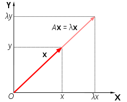 Illustration of a vector {$\mathbf{x}$} that satisfies {$A\mathbf{x} = \lambda\mathbf{x}. \;\; \mathbf{x}$} is simply rescaled (not rotated) by {$A$}. [image from Wikipedia] All non-zero vectors {$\mathbf{v}$} that satisfy such an equation are called eigenvectors of {$A$}, and their respective {$\lambda$} are called eigenvalues. “Eigen” is a German term, meaning “own” (as in “my own” or “self”) or characteristic” or “peculiar to”, which is appropriate for eigenvectors and eigenvalues because to a great extent they describe the characteristics of the transformation that a matrix represents. In fact, for every real-valued, symmetric matrix we can even write the matrix entirely in terms of its eigenvalues and eigenvectors. Specifically, for an {$m \times m$} matrix {$A$} we can state {$A = V \Lambda V^T$}, where each column of {$V$} is an eigenvector of {$A$} and {$\Lambda$} is a diagonal matrix with the corresponding eigenvalues along its diagonal. This is called the eigendecomposition of the matrix. If you want to find some function {$f(A)$} of a matrix {$A$}, e.g {$e^A$}, how would you do it? Some functions are easy {$A^2$}. others not so. All are easy if {$A$} is a diagonal matrix — just apply the function to each element of the diagonal. SImilarly, to ask is a matrix is “positive”, we could ask if all the elements of its diagonal are positive. How do we do this for a general (or for now a general symmetric) matrix? Answer: do a eigendecomposition. Find the solutions to {$A\mathbf{v_j} = \lambda_j\mathbf{v_j}$}, then assemble the eigenvectors {$\mathbf{v_j}$} into a matrix {$V$} and put the eigenvalues {$\lambda_j$} as elements on the diagonal of a matrix {$\Lambda$}, and then {$A = V \Lambda V^T$}. Now we can apply all of our operations {$f()$} to the eigenvalues as if they were scalars! In practice, most eigenvalue solvers use methods such as power iteration to compute eigenvalues. Let’s see how that works by multiplying some arbitrary vector {$x$} repeatedly by a matrix {$A$}. What will {$A A A A A A A x$} approach? Answer: a constant times the eigenvalue corresponding to the largest eigenvalue {$\lambda_1$} How do we know? Answer: write {$x$} in terms of the basis vectors {$v_i$}, by projecting it on to each of them. {$x = \sum_i <x,v_i> v_i$} How fast will it become “pure”? Each multiplication will increase the component of {$v_1$} relative to {$v_2$} by a factor of {$\lambda_1 / \lambda_2$} SVD (singular value decomposition)One can generalize eigenvalues/vectors to non-square matrices, in which case they are called singular vectors and singular values. The equations remain the same, but there are now both left and right singular values and vectors. {$A^TA\mathbf{v} = \lambda\mathbf{v}$} {$ AA^T \mathbf{u} = \lambda\mathbf{u}$} {$A = U \Lambda V^T$}. where {$A$} is {$n*p$},{$U$} is {$n*n$}, {$\Lambda$} is {$n*p$}, and {$V^T$} is {$p*p$}, but {$U$} and {$V$} can be at most rank {$min(n,p)$}, so one of them will have {$n-p$} or {$p-n$} zero eigenvalues. Exercise: show that the nonzero left and right singular values are identical. Any matrix can be decomposed into a weighted sum of it’s singular vectors (giving a singular value decomposition). In practice, we often don’t care about decomposing {$A$} exactly, but only approximating it. For example, we will often take {$A$} to be our “design matrix” of observations {$X$}, and approximate it by the thin SVD obtained when one only keeps the top {$k$} singular vectors and values. {$A \sim U_k \Lambda_k V_k^T$} where {$A$} is {$n*p$}, {$U_k$} is {$n*k$}, {$\Lambda_k$} is {$k*k$}, and {$V_k^T$} is {$k*p$} The thin SVD gives the best rank {$k$} approximation to a matrix, where “best” means minimum Frobenious norm, which is basically the {$L_2$} norm of the elements of the matrix (i.e., the square root of the sum of the squares of all the elements of the matrix, which magically equals the sum of the squares of the singular values). This is often useful. Consider a matrix {$A$} where each student is a row, and each column is set of test result for that student (e.g. a score on an exam question, or to an IQ test, or anything. (More generally, rows are observations, and columns are features.) We can now approximate the student grades by {$\hat{A} \sim U_k \Lambda_k V_k^T$}. Here we have approximated each original {$p$}-dimensional vector by a {$k$}-dimensional one, called the scores. Each student’s grade vector {$x$} can be written in terms of a weighted combination of the basis vectors {$V_k$}. The weights are the “scores”, and the components of the basis vectors are called the loadings of the original features. For example, in a battery of tests of intellectual abilities, the score on the “largest singular vector”—which means the singular vector corresponding to the largest singular value — after all, all the singular vectors have been normalized to be of length 1—is often called g, for “general intelligence”. Why is all this useful? We’ll see many examples over the next couple classes, but here are a few:
but is sometimes a little better — or a little worse. Generalized inversesLinear regression requires estimating {$w$} in {$y = Xw$}, which can be viewed as computing a pseudo-inverse (or “generalized inverse”) {$X^+$} of {$X$}, so that {$w = X^+y$} Thus far, we have done this by {$X^+ = (X^TX)^{-1} X^T$} But one could also compute a generalized inverse using the SVD decomposition {$X^+ = (U \Lambda^{-1} V^T)^T = V \Lambda^{-1} U^T$} then {$X X^+= U \Lambda V^T V \Lambda^{-1} U^T= U U^T=I$} if {$U$} and {$V$} are orthonormal and {$\Lambda$} is invertible. similarly, {$ X^+ X = V \Lambda U^T U \Lambda^{-1} V^T= V V^T=I$} Note that {$ U^T U =U U^T = I$} and similarly with {$V$}. But {$\Lambda$} is often not invertible — since it is, in general, rectangular. So we use a “thin SVD” {$X^+ = V_k \Lambda_k^{-1} U_k^T$} In the thin SVD, we only keep {$k$} nonzero singular values, so that inverse {$\Lambda^{-1}$} is well-defined Fast SVD (Randomized singular value decomposition)This is an extremely useful algorithm that shows how one really does SVD on big data sets. Input: matrix {$A$} of size {$n \times p$}, the desired hidden state dimension {$k$}, and the number of “extra” singular vectors, {$l$}
Output: The left and right singular vectors {$U_{final}$}, {$V_{final}^T$}
Practice exercises
|