|
Lectures /
Math ReviewOn this page… (hide) Machine learning relies on two basic areas of mathematics: linear algebra and probability. This lecture is a brief review of both of these subjects that you are expected to go over on your own. If you feel that you need more practice, a good book for matrices and linear algebra is Matrix Analysis and Applied Linear Algebra by Carl D. Meyer, and a good book for probability is A First Course in Probability, by Sheldon Ross. Any other books that you are comfortable with are fine, as this course simply uses the information in the books, and does not teach them. NOTE If the topics covered in this review are entirely new to you, we STRONGLY urge you to reconsider taking this class! Either drop the course, or take an incomplete and finish it later; the material in this section is only a review, it is not intended to teach you the material for the first time. Matrices and Linear AlgebraOne description of Machine Learning is that it is fancy curve fitting; you have one or more linear equations that can make a prediction of some kind based on some number of inputs. For the moment, we’re going to sidestep how you choose the linear equations that you choose, their coefficients, etc., and concentrate only on what you do once you have them (the bulk of the course is finding those linear equations and their coefficients, so you’ll see all that soon enough). So, let’s jump in: {$ \mathbf{y = X w } $} Thus far, this is exceedingly uninformative. Let’s break it down into its parts to see what is going on.
So another way of looking at {$ \mathbf{y = X w} $} is: {$ \left[\begin{array}{c} y_1 \\ y_2 \\ y_3 \\ \vdots \\ y_n \end{array}\right] = \left[\begin{array}{ccccc} X_{11} & X_{12} & X_{13} & \ldots & X_{1m} \\ X_{21} & X_{22} & X_{23} & \ldots & X_{2m} \\ X_{31} & X_{32} & X_{33} & \ldots & X_{3m} \\ \vdots & \vdots & \vdots & \vdots\;\vdots\;\vdots & \vdots \\ X_{n1} & X_{n2} & X_{n3} & \ldots & X_{nm} \end{array}\right] \times \mathbf{w} $} {$ \mathbf{w} $} is the most interesting part of the stuff above. We know we have some set of inputs, and we have some set of outputs we’re interested in. We think that there is a relation between the two. We need {$ \mathbf{w} $} to be an accurate representation of this relation. Let’s start with the simplest relation we can define. The simplest one is to copy some input variable to the output. So we choose one and do so: {$ y_1 = X_{11} $} Well, this is a good start, but what if our output {$ y_1 $} is dependent on several different inputs, like how today’s weather is dependent on the temperature of the past several days, the humidity, etc. Clearly, a better approximation is a combination of functions: {$ y_1 = X_{11} + X_{12} + X_{13} + \ldots $} So far, so good. But what happens if we try to predict the humidity next using the same set of equations? {$ y_2 = X_{21} + X_{22} + X_{23} + \ldots $} Well, we’re giving the same weights to each of the inputs, which is problem because humidity is measured by percentage and has to be restricted to the values [0.0, 100.0], whereas the temperature in some parts of the world go over 100.0. This is a problem, not just because the output might be out of range, but also because the importance of the incoming input variables might be different depending on what we’re trying to predict. It’d be best if we can scale the weight of the inputs individually: {$ y_2 = X_{21} w_1 + X_{22} w_2 + X_{23} w_3 + \ldots $} Regression explanation {$ \begin{array}{ccccccccc} y_1 & = & X_{11} w_1 & + & X_{12} w_2 & + & \ldots & + & X_{1m} w_m \\ y_2 & = & X_{21} w_1 & + & X_{22} w_2 & + & \ldots & + & X_{2m} w_m \\ \vdots & = & \vdots & + & \vdots & + & \vdots\;\vdots\;\vdots & + & \vdots \\ y_n & = & X_{n1} w_1 & + & X_{n2} w_2 & + & \ldots & + & X_{nm} w_m \end{array} $} Now we have a way of controlling the influence of any particular function and input on any particular output value. But… we’re lazy. We keep repeating the same {$w_1, \cdots, w_m$} on each line, and it’d be nice if there was a simple method of avoiding writing them over and over again. In short: {$ \left[\begin{array}{c} y_1 \\ y_2 \\ y_3 \\ \vdots \\ y_n \end{array}\right] = \left[\begin{array}{ccccc} X_{11} & X_{12} & X_{13} & \ldots & X_{1m} \\ X_{21} & X_{22} & X_{23} & \ldots & X_{2m} \\ X_{31} & X_{32} & X_{33} & \ldots & X_{3m} \\ \vdots & \vdots & \vdots & \vdots\;\vdots\;\vdots & \vdots \\ X_{n1} & X_{n2} & X_{n3} & \ldots & X_{nm} \end{array}\right] \times \left[\begin{array}{c} w_{1} \\ w_{2} \\ \vdots \\ w_{m} \end{array} \right] $} If you notice, the matrix has {$n$} rows and {$m$} columns. By choosing to make the matrix like this, we can have a different number of inputs and outputs, which could be very handy. While we’re at it, we can also see how the matrices and vectors multiple against one another. The matrix rows are multiplied against the input column producing the output {$ y_i = [X]_{i*}*w $}. This is the basics of matrix multiplication. A few things to notice about multiplying to matrices together. If the first matrix has {$k$} rows and {$l$} columns, the second matrix must have {$l$} rows, and {$m$} columns. This should be obvious from the example above; if the number of columns in {$\mathbf{X}$} was not the same as the number of rows in {$\mathbf{w}$} then either there would be too many coefficients or not enough coefficients, which would make the multiplication illegal. ExamplesHere are a couple of worked examples: {$\left[\begin{array}{ccccccccc} 1 & 2 & 3 \\ 4 & 5 & 6 \\ 7 & 8 & 9 \\ \end{array} \right] \times \left[\begin{array}{c} 1 \\ 2 \\ 3 \end{array}\right] = \left[\begin{array}{c} 1*1 + 2*2 + 3*3 \\ 4*1 + 5*2 + 6*3 \\ 7*1 + 8*2 + 9*3 \end{array}\right] = \left[\begin{array}{c} 14 \\ 32 \\ 50 \end{array}\right]$} {$\left[\begin{array}{ccccccccc} 1 & 2 & 3 \\ 4 & 5 & 6 \\ 7 & 8 & 9 \\ 10 & 11 & 12 \\ \end{array} \right] \times \left[\begin{array}{c} 1 \\ 2 \\ 3 \end{array}\right] = \left[\begin{array}{c} 1*1 + 2*2 + 3*3 \\ 4*1 + 5*2 + 6*3 \\ 7*1 + 8*2 + 9*3 \\ 10*1 + 11*2 + 12*3 \end{array}\right] = \left[\begin{array}{c} 14 \\ 32 \\ 50 \\ 68 \end{array}\right]$} Eigenfunctions, Eigenvectors, (eigenfaces, eigenfruit, eigenducks,…)Need to put in an explanation is why they are useful here Get this from Jenny’s lecture ProbabilityThere are many techniques in Machine Learning that rely on how likely an event is to occur. You might want to know if two things relate in some way; perhaps when event {$A$} occurs, {$B$} generally follows. Or you might want to simplify your model, allowing a certain amount of error, in which case you need to know how likely an event is. All of this is part of the field of probability and statistics. To start out with, we need to define some terms, for which it will be simpler if we have some kind of example. So, imagine you have an oddly shaped stone, with some number of faces on it, like so: 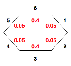 A strangely shaped stoned, used as a die. The black numbers are the values of the 6 faces of the stone, and the red numbers are the probability that the stone will land with that face facing upwards on any given toss. The sample space consists of the set of possible values (the numbers 1–6), and the probability associated with each face being face-up (the red numbers). The sum of all of the probabilities equals 1; this corresponds to the fact that when we toss the stone, some side will end up face-up, although we don’t know which side. Because the stone has no memory (it doesn’t record past tosses), every toss we make is independent of any other toss. In addition, unless the stone suddenly changes shape or something else drastic happens, the probabilities will remain identical. If we toss the stone many times, recording how often each number comes up, we’ll have a distribution of values. These facts together form the term Independent Identical Distribution (often referred to as i.i.d) You’ll see mention that a distribution either is, or is assumed to be i.i.d. quite often in the notes; this is because if we have data that is NOT i.i.d., the computational complexity rises sharply, becoming intractable for all but the smallest of cases. When we toss the stone, we’re often looking for something more complex than just a single face coming up. We might be interested in how likely it is that all even numbered faces come up in 3 consecutive throws, or how likely it is that a 1 or a 6 come up next. Any situation we can pose, even the simple ones of a particular face coming up, is an event. Events are what we’re interested in, but since we only know the probability of the most basic of events, we need to figure out how to combine their probabilities to find the probability of more complex events. Random VariablesRandom variables are horribly named; they are neither random, nor are they variables. They are functions over the sample space. Effectively, they are events. Their set of inputs is the various atomic events, and they output something based on them. For example, you might count how many times the number 3 turns up on a throw of a die in 10 throws. Note that this is not a probability; it is an actual count of some actual set of 10 throws. So, you might get 0 one time, 3 the next, and 10 some other time. In short, it’s just a function, and like any function, it has a well-defined output for some well-defined inputs. Since a random variable is just a function, we can actually do probabilities over it; for example, define a function accepts 10 numbers, each in the range [1,6]. The function adds all the numbers together, and then calculates the square root. What is the probability that the result will be an integer? Or, we can ask if two random variables are independent of one another. Probability studies random variables which are probabilistic outcomes such as a coin flip. The outcome depends on a known or unknown probability distribution. Random variables take values in a sample space, which may be discrete or continuous. The sample space for a coin flip consists of {H, T}. The sample space for temperature can be {$(-\infty, \infty)$} . The number of occurrences of an event would be {1,2,3, . . . } Sample spaces can be defined according to needs by setting upper or lower limits. Instead of saying the sample space for temperature is {$(-infty,\infty) $}, we can specify the range we are experimenting in such as {$ (-300\,^{\circ}{\rm C} , 3000\,^{\circ}{\rm C} )$}. The two sample spaces do not make a difference as long as there is no probability in less than {$ -300\,^{\circ}{\rm C}$} and more than {$ 3000\,^{\circ}{\rm C} $}. Combining EventsUsing the probabilities of the stone described above, what is the probability that either a 1 or 6 come up on any particular toss? The answer is fairly clearly 0.45. But why is it so clearly 0.45? The answer is that each event is disjoint from one another; we can have either a 1 or a 6, but not both. This is an important requirement when combining events. If we don’t take into account the fact the events may overlap, we might have a greater than 1 probability. So let’s look at an example where the events do overlap: What is the probability that the stone’s value on the next toss will be even or a prime number? The probability that it will be even is {$0.05 + 0.05 + 0.4 = 0.5$}, and the probability that it will be prime is {$0.05 + 0.4 + 0.05 = 0.5$}. However, this still leaves out the number 1, which has a probability of 0.05. Clearly, if we add everything together, we’ll get {$0.5 + 0.5 + 0.05 = 1.05 > 1$}, which is illegal. The problem is the number 2; it is both even and a prime. We need to make sure that we don’t count it twice. And so we have the following rule: {$P(A \cup B) = P(A) + P(B) - P(A \cap B)$} In our example, {$A$} is the event that a toss will turn up an even number, and {$B$} is the event that a toss will turn up a prime number. Since both {$A$} and {$B$} count the number 2, we remove one of the copies via {$P(A \cap B)$}. Doing so for the probabilities above, ensures that the total probability will be exactly 1. The equation above is one example of the Inclusion-Exclusion Principle, which, although you won’t see it in use in this class, does affect probability, and therefore indirectly affects this class. Discrete distributionsRandom variables take discrete values which are separate and distinct in a discrete distribution. The variables in such distributions can take a finite number of values. A discrete distribution can have infinite variables and so infinite number of possible values such as the Poisson distribution. For any valid discrete distribution, the probabilities over the atomic events must sum to one; that is, An event is a subset of atoms (one or more). The probability of an event is the sum of the probabilities of its constituent atoms. A distribution may be visualized with the following picture, where an atom is any point inside the box. Those points inside the circle correspond to outcomes for which X = x; those outside the circle correspond to outcomes for which X = x.  Venn diagram representation of a probability distribution for a single random variable Joint distributionsA joint distribution looks at the probability of more than one random variable. If there are only two random variables, this is called bivariate. An example to bivariate distribution will be the probability of getting one tail and one head from two coin flips, which would be ½* ½ = ¼ It is a bivariate distribution because two coins are flipped. If the random variables are more than two, then it is called multivariate distribution. Joint distribution can be represented the way probability distribution for a single random variable is represented. Let’s say X is head and Y is tail:  Conditional ProbabilityOK, so now we know how to combine different events together to generate more interesting events. But the combinations that we’ve got are essentially just unions or intersections of different events; what happens if we already know that a particular event occurred, and given that information want to know what the probability of a second event occurring is? E.g., if someone tells me that on the last stone’s throw, the value was a prime number, what is the probability that it was also an even number? Let’s reason it out. Call the event that the stone is prime {$A$} and the event that it is even {$B$}. Since there is only one number in this event, and that number is 2, we already know what the probability of the event is, when we don’t know anything else. That value is 0.05, the probability that a 2 will turn up. But since we already know that the value was a prime number, there are only 3 values it could be: {2,3,5}. So, given this information, the probability that the value will be a 2 given that is prime is: {$\mbox{Probability of 2 given A = } P(2|A) = \frac{P(2)}{P(A)} = \frac{0.05}{0.5} = 0.1$} Put in a slightly more abstract form, if we have two events {$A$} and {$B$}, and we know that event {$B$} has a non-zero probability, then the probability that {$A$} will happen if {$B$} has already happened is: {$P(A|B) = \frac{P(A \cap B)}{P(B)}$} Note that it is common to see {$P(A \cap B)$} as {$P(AB)$}. DO NOT allow yourself to think it means {$P(A) \times P(B)$}! By that logic, the probability that the stone will turn up as a 3 and a 6 at the same time is 0.16, which is clearly impossible. Manipulating distributionsBayes RuleOK, so at this point, we can calculate the probability of event {$A$} happening if we know that event {$B$} has already happened. But what happens if we want to know the exact opposite? That is, instead of {$P(A|B)$}, we want {$P(B|A)$} when what know is {$P(A|B)$}, {$P(A)$}, and {$P(B)$}? Well, let’s start with what we know: {$P(A|B) = \frac{P(A \cap B)}{P(B)} \longrightarrow P(A \cap B) = P(A|B) P(B)$} {$P(B|A) = \frac{P(A \cap B)}{P(A)} \longrightarrow P(A \cap B) = P(B|A) P(A)$} Combining terms, we get: {$P(A \cap B) = P(A|B) P(B) = P(B|A) P(A)$} Which, with a little algebra is: {$P(B|A) = \frac{P(A|B) P(B)}{P(A)}$} This is known as Bayes Rule or Bayes Theorem (also see wikipedia), and is useful in those cases where you know (or it is easy to get) all the parts on the right hand side, but very difficult to get the part on the left hand side. Note that we will be using this in class a great deal, so the more you understand it and how to apply it now, the more likely it is that you will pass the class and the qualifier. The chain ruleThe chain rule lets us define the joint distribution of more than one random variables as a product of conditionals: {$ P(X,Y) = \frac {P(X,Y)} {P(Y)} P(Y) = P(X|Y) P(Y)$} We can derive the unknown P(X,Y) with the chain rule. The chain rule can be used with any N number of variables and the random variables can be in any order. {$ P(X_{1}, . . . , X_{N}) = \prod_{n=1}^N P(X_{n}|X_{1},..., X_{n-1}) $} MarginalizationIn a given a collection of random variables, we are often interested in only a subset of them. For example, we might want to compute {$ P(X) $} from a joint distribution {$ P(X, Y, Z)$}. Marginalization allows us to compute {$ P(X) $} by summing over all possible combinations of the other variables. Marginalization derives from the chain rule. Marginal probability is the unconditional probability {$ P(A) $} of the event A,whether the event B occurred or not. Given the outcome of the random variable X, the marginal probability of even A is the summation of joint probabilities of all outcomes of X. If X has two outcomes B and B’, then {$ P(A)= P(A \cap B) + P(A \cap B') $}
Note: To see an example of marginalization, look at the last problem in the self test and its solution. Structural PropertiesIndependenceX is independent of Y means that knowing Y does not change our belief about X.
Conditional IndependenceRandom variables are rarely independent but we can still use local structural properties such as conditional independence.
The following should hold for all x,y,z:
ExamplesBayes Rule can have very surprising results sometimes. Here are some examples that illustrate how strange some of the results you get can be: The Two Child Problem asks the following question: I have two children, at least one of whom is a son. What is the probability that both children are boys?
At first glance, it appears that the probability that the other child is a boy is {$\frac{1}{2}$}; after all, what does the sex of one child have to do with the other? Unfortunately, everything. Here is a table of the possible family makeups:
So the probability that both children are boys is {$\frac{1}{3}$}. Now let’s redo this using Bayes rule. Let {$P(B)$} be the probability that at least one child is a boy. Since this occurs in {$\frac{3}{4}$} cases, {$P(B) = \frac{3}{4}$}. Let the probability that both children are boys be {$P(BB) = \frac{1}{4}$}. Finally, we know that {$P(B|BB) = 1$}; this makes sense because it says that if we know both children are boys, than the probability that at least one is a boy is 1. So, combining everything together: {$P(BB|B) = \frac{P(B|BB) P(BB)}{P(B)} = \frac{1 \times\frac{1}{4}}{\frac{3}{4}} = \frac{1}{3}$} The Tuesday Child Problem Now for a more difficult problem; the Tuesday Child Problem. The problem is this: I have two children, at least one of whom is a son born on a Tuesday. What is the probability that I have two boys?
At first glance, it appears that the fact that one of the children is a son, and that he is born on a Tuesday, is unimportant. From the Two Child Problem, know that the fact that one child is a boy is actually important. The really strange part is the fact that that child is also born on a Tuesday is also important. Here’s why: Assume for the moment that the older child was the boy that was born on Tuesday. Then there are 14 possibilities for the younger child; he or she could be a boy or a girl, and could have been born on any day of the week. Half of those possibilities include a boy. So, 7 ‘good’ events out of 14 possible. Now for the younger child. Assume the younger child was the one born on a Tuesday. What are the possible, allowable states for the older child? As it turns out, the older child can be any combination except a boy born on a Tuesday. This is because the case of the older child being a boy born on a Tuesday was already handled in the first case, and counting it a second time would be double counting (Have a look at the picture of the states, and see the section on Combining events if you’re confused by this). Thus, there are 13 cases where the younger child is a boy born on a Tuesday, and only 6 of these cases are where the older child is a boy. So, 6 of the 13 events are ‘good’. Combining the two together yields {$\frac{7 + 6}{14 + 13} = \frac{13}{27}$}. Now using Bayes Rule (see the picture for help with this)  The Tuesday Child Problem, visually demonstrated First off, we need to decide what events are important to us. These are the following:
So now we need to start calculating probabilities: {$ \; $ \begin{align*} P(BB) & = P(BG) = P(GB) = 1/3 \\ P(GG) & = 0 \end{align*} $ \; $} Note that the numbers above are exactly what we’d expect from the Two Child Problem. Now things get more interesting; we need to calculate the conditional probability that at least one child is a son born on a Tuesday given that the children are BB, BG, GB, or GG. {$ \; $ \begin{align*} P(B|BB) & = \frac{13}{49} \\ P(B|BG) & = \frac{1}{7} \\ P(B|GB) & = \frac{1}{7} \end{align*} $ \; $} Note that calculating {$P(B|GG)$} doesn’t make any sense because we know that {$P(GG) = 0$}. So we just leave that part out. Next, we need to calculate {$P(B)$}. This is just the average of {$P(B|BB)$}, {$P(B|BG)$}, {$P(B|GB)$}: {$ \; $ \begin{align*} P(B) & = \frac{\frac{13}{49} + \frac{1}{7} + \frac{1}{7}}{3} = \frac{9}{49} \end{align*} $ \; $} We finally have all the parts we need to use Bayes Theorem: {$P(BB|B) = \frac{P(B|BB) \times P(BB)}{P(B)} = \frac{\frac{13}{49} \times \frac{1}{3}}{\frac{9}{49}} = \frac{13}{27}$} Note that {$\frac{13}{27} \approx \frac{1}{2}$}, which is quite different from the answer to the Two Child Problem. If this is not a surprising result to you, I’ll be honest, it is an astonishing result to me! Monty Hall Problem The Monty Hall Problem is yet another strange application of probability. The Monty Hall Problem asks the following question: You are in a game given three doors as a choice. There are goats behind two of the doors and behind the other, a car. You are trying to find the car. You pick one of the doors and the host of the game opens another door for you which has a goat. The host asks you if you want to change your first choice. Is switching your choice to your advantage?
Most of the time our mind tricks us to think that they are all equally probable, so since one door with a goat is open, the chances to find the car in both doors is {$\frac{1}{2}$}; which is incorrect. Switching your choice will double your probability of finding the car. You first choice had {$\frac{1}{3}$} probability of hiding the car. The two other doors have a total probability of {$\frac{2}{3}$}. When one of the doors with a goat is open, that still preserves the probability. So the door that you didn’t choose will have 2/3 probability of hiding the car. This can be proven by Bayes Theorem. C is the number of the door with the car. S is the number of the door selected by the player. H is the door opened by the host that hides a goat. The probability is unconditional. {$ \; $ \begin{align*} P(C) & = \frac{1}{3} \\ P(S) & = \frac{1}{3} \\ P(H) & = \frac{1}{3} \end{align*} $ \; $} Player’s initial choice is independent therefore conditional probability of C given S is: {$ \; $ \begin{equation*} P(C|S) = P(C)\end{equation*} $ \; $} Since the host knows what is hidden behind each door, the conditional probability given C and S is:
After the player selects a door and the host opens one, the player can calculate the probability of C given H and S. {$ \; $ \begin{equation*} P(C|H,S) = \frac {P(H|C,S)P(C|S)}{P(H|S)} \end{equation*} $ \; $} We know that {$P(H|C,S) = 1$} and {$P(C|S) = P(C) = \frac {1}{3}$} The denominator which is the marginal probability is: {$ \; $ \begin{equation*} P(H|S) = \sum _{C=1}^3 P(H,C|S) = \sum _{C=1}^3 P(H|C,S)P(C|S) \end{equation*} $ \; $} Let’s say the car is behind door 1, the player selects door 2 and the host opens door 3; the probability of winning by switching will be: {$ \; $ \begin{equation*} P(C=1|H=3,S=2) = \frac { 1 \times \frac{1}{3} } { \frac{1}{2} \times \frac{1}{3} + 1 \times \frac{1}{3} + 0 \times \frac{1}{3} } = \frac {2}{3} \end{equation*} $ \; $} |