|
Lectures /
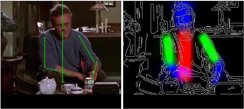
Bayes NetsOn this page… (hide) Directed Graphical Models: Bayes NetsProbabilistic graphical models represent a joint distribution over a set of variables. {$P(X_1,\ldots,X_m)$} Given a joint distribution, we can reason about unobserved variables given observations (evidence). Here’s an applet (model file: http://www.cs.cmu.edu/~javabayes/Examples/CarStarts/car-starts.bif) that illustrates reasoning with a Bayes Net. Here’s an example from Ben Taskar (with Ben Sapp) of using graphical models for detection and parsing of human figures: 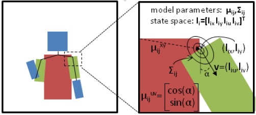 Pictorial Structure model (Bayes net)
 Posterior distribution over head/torso/limbs locations
The Naive Bayes model is an example of a joint distribution model (where one of the variables is the class variable {$Y$}): {$P(Y,X_1,\ldots,X_m) = P(Y)\prod_j P(X_j|Y)$} We used the Naive Bayes model diagnostically: Given the effects (features) {$X_1=x_1,\ldots, X_m=x_m$}, we used Bayes rule to compute {$P(Y|x_1,..,x_m)$}, the posterior over the cause. More generally, the joint distribution allows us to compute the posterior distribution over any set of variables given another set of variables. Representing the JointThe joint distribution of a set of variables is an exponentially-sized object. If all the variables are binary, the joint over {$m$} variables has {$2^m$} −1 parameters. The Naive Bayes model is much more concise: it uses conditional independence assumptions to restrict the types of distributions it can represent and uses {$O(m)$} parameters. The key to concise representation is factoring: representing the whole with a product of interrelated parts. The key ingredients in this representation are the chain rule, Bayes Rule and conditional independence. {$\textbf{Chain Rule}: P(X_1,\ldots, X_m) = P(X_1)P(X_2|X_1)P(X_3|X_2,X_1)\ldots P(X_m|X_1,\ldots,X_{m-1})$}. The chain rule by itself does not lead to concise representation: we need to assume conditional independencies to reduce the size of the representation. Let’s consider some very simple examples. We want to reason about three variables: Traffic (whether there will be traffic on the roads tomorrow), Rain (whether it will rain tomorrow), Umbrella (whether I’ll bring my umbrella with me tomorrow). These random variables are clearly correlated. Using the chain rule, we have: {$P(R,T,U) = P(R)P(T|R)P(U|T,R)$} Now if we assume that my decision about the umbrella does not depend on traffic once I know if it’s raining, i.e. {$P(U|T,R) = P(U|R)$}, then we have {$P(R,T,U) = P(R)P(T|R)P(U|R)$} Conditional Independence: {$X_i$} is conditionally independent of {$X_j$} given {$X_k$}, denoted as {$X_i \bot X_j | X_k$} if {$P(X_i=x_i \mid X_k=x_k, X_j=x_j)= P(X_i=x_i \mid X_k=x_k), \; \forall x_i,x_j,x_k$} or equivalently: {$ \; \begin{align*} & P(X_i=x_i,X_j=x_j\mid X_k=x_k) = \\ & \quad \quad \quad P(X_i=x_i\mid X_k=x_k)P(X_j=x_j\mid X_k=x_k), \; \forall x_i,x_j,x_k \end{align*} \; $}. Graphical models use conditional independence assumptions for efficient representation, inference and learning of joint distributions. The above model for R,T,U can be represented as a directed graph, {$U \leftarrow R \rightarrow T$}, where nodes correspond to variables and edges correspond to direct correlations, which we will define precisely below. Here’s a toy graphical model for a car operation. 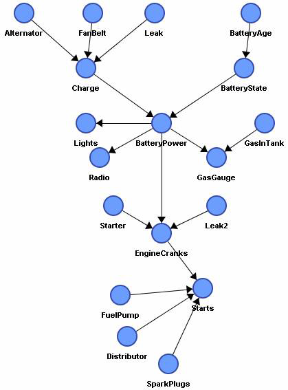
Graphical models are simplified descriptions of how some portion of the world works. They will usually not include every possible variable or all interactions between variables, but focus on the most relevant variables and strongest interactions. Their probabilistic nature allows reasoning about unknown variables given partial evidence about the world. Directed graphical models, know as Bayesian Networks, Bayes Nets, Belief Nets, etc, can be thought of as causal models (with some important caveats). Typically, causal models (if they exist) are the most concise representation of the underlying distribution. There are several types of reasoning we can do with such models:
Graphical Models represent joint distributions using simple, local interactions models which describe how variables depend on each other. Local interactions are then chained together to give global, indirect interactions. In case of directed graphical models (Bayes nets), local interactions are conditional distributions. The graphical representation encodes conditional independence assumptions. Graphs and Conditional Independence AssumptionsLet’s consider a graphical model for a slightly more complex example:
A Bayes net which encodes the assumptions for this example is shown below. Nodes represent variables 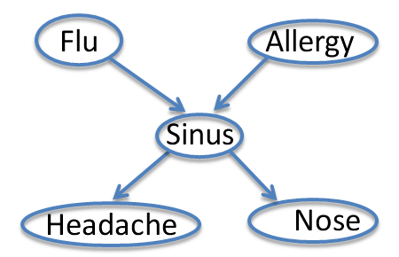 {$P(F,A,S,H,N) = P(F)P(A)P(S|F,A)P(H|S)P(N|S)$}
The graph encodes the following conditional independence assumptions (and more).
Here’s another classic example, due to Judea Pearl, who was instrumental to popularizing Bayes nets and probabilistic reasoning in AI. It helps to know that he lives in LA. John calls to say my house alarm is ringing, but neighbor Mary doesn’t call. Sometimes it’s set off by minor earthquakes. Is there a burglar? The variables are: Burglary, Earthquake, Alarm, JohnCalls, MaryCalls. Our model will reflect the following assumptions:
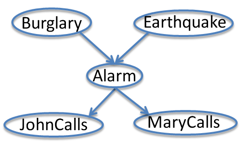 {$P(E,B,A,J,M)= P(E)P(B)P(A|B,E)P(J|A)P(M|A)$}
In general, the graph encodes the following basic assumption, from which many others can be derived: Local Markov Assumption (LMA): A variable X is independent of its nondescendants given its parents (and only its parents) : {$ X \bot NonDescendants_X | Pa_X $} For our purposes here, a node X’ is a non-descendant of X if X’ is not X and not a parent of X and there is no directed path from X to X’. Parameters: Conditional DistributionsThe directed graph encodes independencies. The numerical value of the joint distribution is encoded in local conditional distributions. In case of discrete variables, these are called CPTs (conditional probability tables). 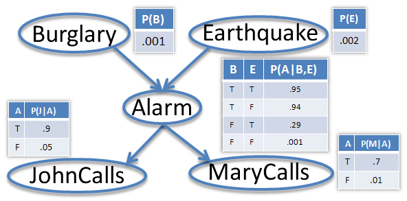 {$P(E,B,A,J,M)= P(E)P(B)P(A|B,E)P(J|A)P(M|A)$}
The Local Markov Assumption allows us to decompose the joint in terms of the CPTs: {$P(E,B,A,J,M) = P(E)P(B|E)P(A|B,E)P(J|A,B,E)P(M|J,A,B,E) = P(E)P(B)P(A|B,E)P(J|A)P(M|A)$} Why? Let’s look at the general case. General Bayes Net Definition
The last statement about the joint distribution is due to the following construction. Take a topological sort of the DAG and renumber the variables such that all the children of a node appear after it in the ordering. Then {$P(X_1,\ldots,X_m) = \prod_j P(X_j | X_{j-1},\ldots,X_1) = \prod_j P(X_j | Pa_{X_j}) $} by LMA: since none of {$j$}’s children appear before {$j$} in the ordering, {$X_{j-1},\ldots,X_1$} only contains its parents and non-descendants. Properties of Conditional IndependenceThe Local Markov Assumption specifies the set of basic independencies in a Bayes net. We can use properties of conditional independence to infer many others. (Proofs follow by noting that {$X \bot Y$} iff {$P(X,Y) = P(X)P(Y)$}.)
{$(X \bot Y | Z) \rightarrow (Y \bot X | Z)$}
{$(X \bot Y,W | Z) \rightarrow (X \bot Y | Z)$} {$(X \bot Y,W | Z) \rightarrow (X \bot Y | Z,W) $}
{$(X \bot W | Y,Z), (X \bot Y | Z) \rightarrow (X \bot Y,W | Z)$}
{$(X \bot Y | W,Z), (X \bot W | Y,Z) \rightarrow (X \bot Y,W | Z)$} Conditional Independence In Bayes NetsFor the Flu-Sinus network, the LMA (plus symmetry and decomposition) gives the following indepedencies:
Explaining AwayUsing the Flu-Sinus network, a reasonable setting of parameters could give: {$P(F=t)=0.1, \;\; P(F=t | A=t)=0.1,\;\; P(F=t | S=t)=0.8, \;\; P(F=t | S=t,A=t)=0.5$} that is {$(F\bot A), \; \neg (F\bot A \mid S)$}. This property of distributions, called explaining away, can be encoded in the V-structures of a Bayes net. The CPTs shown for the Burglar-alarm network above exhibit exactly this explaining away property. 3-Node BNsFor 3 node BNs, there are several possible DAG structures: fully disconnected (1), fully connected (6), partially disconnected (6) and the following 4 cases:
In the first 3 cases, we have {$\neg X\bot Z$} but {$X\bot Z \mid Y$}, and in the fourth, the V-structure, we have {$X\bot Z$} but {$\neg (X \bot Z \mid Y)$} In the first three cases, X influences Z (without observations) but the influence is stopped by observing Y, while in cases like 4, X does not influence Z (without observations) but the influence is enabled by observing Y. In the Flu-Sinus network, observing S correlates F and A because of possible explaining away. More generally, observing any descendant of S correlates F and A since we have evidence about S which could be explained away by one of the causes of S. Active TrailsDefinition: A simple trail {$\{X_1 , X_2 , \cdots, X_k\} $} in the graph (no cycles) is an active trail when variables {$O \subset \{X_1, \cdots, X_m\}$} are observed if for each consecutive triplet in the trail:
Directed Separation (d-sep) Theorem: Variables {$X_i$} and {$X_j$} are independent given {$O \subset \{X_1, \cdots, X_m\}$} if there is no active trail between {$X_i$} and {$X_j$} when variables {$O$} are observed. The same theorem applies for sets of variables A,B: if there are no active trails between any pairs of variables {$(X_i \in A, X_j \in B)$} when {$O$} are observed, then {$(A\perp B | O)$}. Algorithm for evaluating Conditional Independence in Bayes NetsFirst, recall that Bayes nets are encoding exactly the Local Markov Assumption: A variable X is independent of its nondescendants given its parents (and only its parents). In simple cases, this can be applied directly to evaluate conditional independence. In general, the d-sep theorem directly implies the following algorithm. If we want to know if {$A \perp B \; | \; X_1,\dots,X_k$}, then: Identify all the simple paths between A and B (ignoring direction of the arrows). For each one: Go along the path. For each triplet (three consecutive variables, including overlaps) in the path, check if it is active using the d-sep conditions. To do this, note that for the triplet X, Y, Z, there are four possible topologies:
Each of these corresponds to one case in the d-sep theorem. Find the case corresponding to the triplet. The triplet is active if the d-sep condition is satisfied. The entire path is active if and only if every triplet in the path is active. If the path is active, conclude {$\neg (A \perp B \; | \; X_1,\dots,X_k)$}. Otherwise, move on to the next path. If no path is active, conclude {$(A \perp B \; | \; X_1,\dots,X_k)$}. Here are some examples: 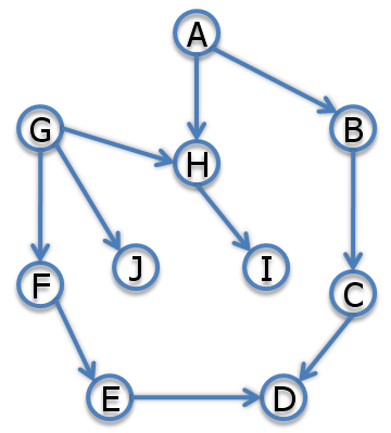 {$(A\bot G),\; (A\bot C | B),\; (A\bot C | B, D),\; \neg (A \bot C \mid B, D, I)$}
Representation TheoremDefinition: {$I(G)$} is the set of all independencies implied by directed separation on graph G. Definition: {$I(P)$} is the set of all independencies in distribution P. BN Representation Theorem {$I(G) \subseteq I(P) \Leftrightarrow P(X_,\ldots,X_m) = \prod_i P(X_i | Pa_{X_i})$} This theorem is important because it tells us that every P has at least one BN structure G that represents it and conversely if P factors over G, then we can read (a subset of) I(P) from G. Back to Lectures |