On this page… (hide)

Alternative derivation of the SVM objective

Suppose we want to learn how to classify a type of data where the output is binary {$y \in \{-1, 1\}$}. We decide to model the data using {$h(\mathbf{x}) = sign(f(\mathbf{x}))$}, where {$f(\mathbf{x}) = \mathbf{w}^\top\mathbf{x} + b$}, a linear separator in the input space {$\mathbf{x}$}. There may be many {$\mathbf{w}$} that can give zero or low error for {$h(\mathbf{x})$}, but intuitively, we want the {$\mathbf{w}$} that makes training points with label {$-1$} have as small {$f(\mathbf{x})$} as possible and those with label {$1$} have as large {$f(\mathbf{x})$} as possible. That is, we want our model to separate the values it assigns to examples with different {$y$} as much as possible. To state this intuition mathematically, we can assign this separation distance a variable name {$d$}, and then the task becomes one of solving the optimization:

{$ \; $ \begin{align*} \max_{\mathbf{w},b,d}\;\; & d \\ \textrm{s.t.}\;\; & f(\mathbf{x}_i) \leq -d \;\;\;\;\;\;\forall i \;\;\textrm{where}\;\; y_i = -1 \\ & f(\mathbf{x}_i) \geq d \;\;\;\;\;\;\forall i \;\;\textrm{where}\;\; y_i = 1. \end{align*} $ \; $}

Note that we can write the constraints more concisely, as simply {$y_i f(\mathbf{x}_i) \geq d \;\;\;\forall i$}, by taking advantage of the fact that {$y_i$} is really just a sign in this case.

The problem with this optimization is that scaling {$\mathbf{w}$} by a positive constant {$c_1$} would increase {$y_i f(\mathbf{x}_i)$}, allowing the constraints {$y_i f(\mathbf{x}_i) \geq d \;\;\;\forall i$} to be satisfied for larger {$d$}. Thus, the solution to the optimization as stated would be to set the weights in {$\mathbf{w}$} to {$\infty$}. Intuitively, this wouldn’t make for a good classifier. To fix this, consider scaling the constraints by {$||\mathbf{w}||_p$}. Since positive homogeneity is a property of norms, we know {$||c_1\mathbf{w}||_p = c_1||\mathbf{w}||_p$}. This means that the constraint {$y_i f(\mathbf{x}_i) / ||\mathbf{w}||_p \geq d$} won’t allow {$d$} to increase for scalings of {$\mathbf{w}$}.

This change in the constraints avoids the bad case where the weights {$\mathbf{w}$} get set to {$\infty$}, but our objective is not yet perfect. It has redundant variables. That is, {$d$} and {$\mathbf{w}$} are too closely related. To fix the problem, we can eliminate the redundancy by requiring {$d ||\mathbf{w}||_q = c_2$} for some positive constant {$c_2$}. This effectively gives the optimization a budget on the product {$d ||\mathbf{w}||_q$}. Maximizing {$d$} subject to this constraint is the same as maximizing {$c_2 / ||\mathbf{w}||_q$}, so we can replace all {$d$} with this value:

{$ \; $ \begin{align*} \max_{\mathbf{w},b}\;\; & \frac{c_2}{||\mathbf{w}||_q} \\ \textrm{s.t.}\;\; & \frac{y_i f(\mathbf{x}_i)}{||\mathbf{w}||_p} \geq \frac{c_2}{||\mathbf{w}||_q} \;\;\;\forall i \end{align*} $ \; $}

If we simply make a few cosmetic changes to the way this is written, changes that won’t affect the location of the separating line that is learned, this optimization problem will look exactly like the SVM primal from lecture. Specifically, let’s:

Select {$c_2 = 1$}. It’s an arbitrary constant that only controls the scale of {$\mathbf{w}$}. The line {$\mathbf{w}^\top\mathbf{x} + b = 0$} is the same as the line {$10000*(\mathbf{w}^\top\mathbf{x} + b) = 0$}. (Try plotting them if you don’t believe it.)
Invert the expression {$\max_{\mathbf{w},b,d}\;\; d = \max_{\mathbf{w},b,d}\;\; c_2 / ||\mathbf{w}||_q$} to get {$\min_{\mathbf{w},b,d}\;\; ||\mathbf{w}||_q / c_2$}. Maximizing an expression is equivalent to minimizing its inverse.

Now our optimization is:

{$ \; $ \begin{align*} \min_{\mathbf{w},b}\;\; & ||\mathbf{w}||_q \\ \textrm{s.t.}\;\; & y_i f(\mathbf{x}_i) \frac{||\mathbf{w}||_q}{||\mathbf{w}||_p} \geq 1 \;\;\;\forall i \end{align*} $ \; $}

If {$q = p = 2$}, we recover almost exactly the SVM primal from lecture. The only other cosmetic change we have to make to achieve exactly the expression from lecture is to square the objective, converting {$||\mathbf{w}||_2$} to {$||\mathbf{w}||_2^2 = \mathbf{w}^\top\mathbf{w}$}. Squaring doesn’t change the {$\mathbf{w}$} at which the maximum is achieved since {$||\mathbf{w}||_2$} is always a non-negative number already.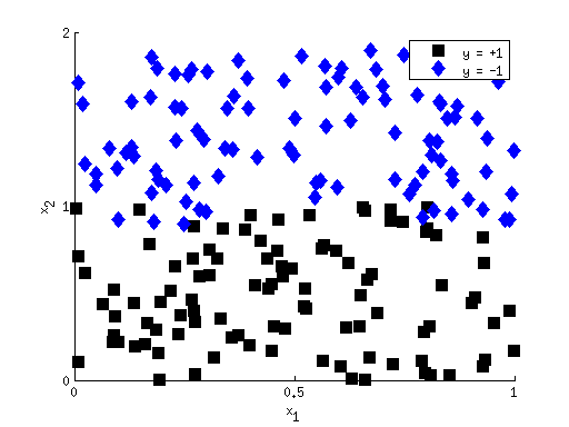

While the standard SVM uses {$q = p = 2$}, other norms have some interesting properties. In particular, using {$q = 1$} may be advantageous when there are redundant noise features. For instance, consider if there are two features {$x_1$} and {$x_2$}, but {$x_1$} is unimportant, as in the figure on the left. Ideally, we would like the SVM to learn {$w_1 = 0$}. In the {$q = 2$} objective, the cost paid for non-zero {$w_1$} is {$w_1^2$}, while for {$q = 1$} the penalty is {$|w_1|$}. For small {$w_1$} ({$w_1 < 1$}), the penalty is larger in the {$q = 1$} case. This makes it more likely that using {$q = 1$} will drive the weights of irrelevant features to zero.

Derivation of the non-separable dual

To the lecture notes!

Proof SVM primal and dual are quadratic programs

Both the SVM primal and dual are quadratic programs (QPs). That is, they are of the form:

{$ \; $ \begin{align*} \min_{\mathbf{z}}\;\; & \mathbf{z}^\top Q\mathbf{z} + \mathbf{c}^\top\mathbf{z} \\ \textrm{s.t.}\;\; & A\mathbf{z} \leq \mathbf{g},\;\; E\mathbf{z} = \mathbf{d} \end{align*} $ \; $}

for some matrices {$Q$}, {$A$}, {$E$} and vectors {$g$}, {$d$}.

Recall the SVM primal:

{$ \; $ \begin{align*} & \textbf{Hinge primal:} \\ \min_{\mathbf{w},b,\xi\ge0}\;\; & \frac {1}{2}\mathbf{w}^\top\mathbf{w} + C\sum_i\xi_i \\ \textrm{s.t.}\;\; & y_i(\mathbf{w}^\top\mathbf{x}_i + b) \ge 1-\xi_i, \;\;\ i=1,\ldots,n \end{align*} $ \; $}

Let the vector {$\mathbf{z}$} from the general quadratic program definition stand for the concatenation of the {$\mathbf{w}$} vector, the variable b, and a vector of all the {$\xi_i$}, {$\mathbf{\xi} = [\xi_1, \ldots, \xi_n]^\top$}. Assuming there are {$n$} training points and {$m$} features, then we have:

{$\mathbf{z} = \left[\begin{array}{c} \mathbf{w} \\ b \\ \mathbf{\xi} \end{array}\right],\;\;\;\; Q = \left[\begin{array}{cc} I_{m \times m} & \mathbf{0}_{m \times (n+1)} \\ \mathbf{0}_{(n+1) \times m} & \mathbf{0}_{(n+1) \times (n+1)} \end{array}\right],\;\;\;\; \mathbf{c} = \left[\begin{array}{c}\mathbf{0}_{(m+1) \times 1} \\ \mathbf{C}_{n \times 1} \end{array}\right]$}

The constraints also fit into the general quadratic program form. The matrix {$A$} will be size {$n \times (m + 1 + n)$}, with one row {$A_i$} for each constraint:

{$A_i = -1 * \left[y_i x_{i1},\; y_i x_{i2},\; \ldots,\; y_i x_{im},\; 1,\; \mathbf{0}_{1 \times (i - 1)},\; 1,\; \mathbf{0}_{1 \times (n - i)}\right]$}

and corresponding {$\mathbf{g} = \mathbf{-1}_{n \times 1}$}. Since we have no equality constraints in the SVM primal, {$E$} and {$\mathbf{d}$} can be considered to be simply zero.

Similarly, we can also show that the dual is a quadratic program by fitting it into the general form. Recall the SVM dual:

{$ \; $ \begin{align*} & \textbf{Hinge kernelized dual:} \\ \max_{\alpha\ge 0}\;\; & \sum_i \alpha_i - \frac{1}{2}\sum_{i,j} \alpha_i\alpha_j y_i y_jk(\mathbf{x}_i,\mathbf{x}_j) \\ \textrm{s.t.}\;\; & \sum_i \alpha_i y_i = 0,\;\; \alpha_i\le C,\;\; i=1,\ldots,n\end{align*} $ \; $}

This time, let the vector {$\mathbf{z}$} from the general quadratic program definition just stand for the {$\alpha$} vector {$[\alpha_1, \ldots, \alpha_n]^\top$}. Then we have:

{$\mathbf{z} = \alpha,\;\;\;\; Q_{ij} = y_i y_j k(\mathbf{x}_i, \mathbf{x}_j),\;\;\;\; \mathbf{c} = \mathbf{1}_{n \times 1}$}

where {$Q$} is size {$n \times n$}. Again, the constraints also fit into the general quadratic program form. The matrix {$A$} will be size {$2n \times n$}, with one row {$A_i$} for each constraint. If we let the first {$n$} rows code for the upper bounds {$\alpha_i \leq C$} and the remaining {$n$} code for the lower bounds {$0 \leq \alpha_i$}, then:

{$A = \left[\begin{array}{c} I_{n \times n} \\ -I_{n \times n} \end{array}\right],\;\;\;\; \mathbf{g} = \left[\begin{array}{c} \mathbf{C}_{n \times 1} \\ \mathbf{0}_{n \times 1} \end{array}\right]$}

For the dual, {$E$} and {$\mathbf{d}$} are also relevant, but simple since there is only a single equality constraint. {$E$} is just an {$1 \times n$} vector of the {$y_i$}, and {$\mathbf{d}$} is a single zero.

The fact that both the primal and dual are quadratic programs allows us to reason about them using established facts about the general class of quadratic programming problems. Most importantly, the literature on quadratic programming states that if {$Q$} is a positive semi-definite (PSD) matrix then the optimization problem is convex. We learned in the kernels lecture that all kernel matrices are PSD, so this assures us that the SVM primal and dual are convex. The good thing about convex functions is that they have no local minima that aren’t also global minima. That is, if we follow their gradient, we will eventually reach a global minimum.

Sequential minimal optimization (SMO)

To solve the SVM problem in the primal form, it is relatively efficient to use gradient-descent-based methods. For an example algorithm, check out this paper which details a gradient descent algorithm for SVMs, PEGASOS, in its first figure.

But in practice, we usually want to optimize the dual, since it:

Allows kernalization, which often means we can get a large number of features at a fraction of the cost of explicitly computing these features. See the kernel trick lecture notes for a reminder example of this type of computation-saving.
Gives a decision rule {$h(\mathbf{x}) = sign(\sum_{i \in SV} \alpha_i y_i k(\mathbf{x_i}, \mathbf{x}))$} that can be much faster to evaluate than the equivalent {$h(\mathbf{x}) = sign(\mathbf{w}^\top\phi(\mathbf{x}) + b)$} when there are many features but few support vectors. (SV here is the set of points that are support vectors; recall that only the support vectors have non-zero {$\alpha_i$}.)

Since the dual is also a convex quadratic program, we could of course solve it using gradient-descent-based methods also. However, there are a number of specialized algorithms for solving it that tend to be more efficient. One of the most common such specialized methods is called sequential minimal optimization (SMO). At a high level, the way SMO works is that it operates on just two {$\alpha_i$} at a time, executing a form of coordinate descent. That is, instead of doing gradient descent on all the variables at once, it works with just two of them at a time but is still able to guarantee convergence to the optimum.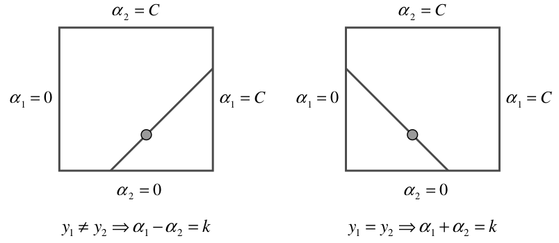

Why does SMO operate on two variables at a time instead of, even simpler, just one? The issue there is that if the {$\sum_i \alpha_i y_i = 0$} constraint is satisfied, then we can’t modify just a single {$\alpha_i$} without violating this constraint. We have to change at least two of them. The diagonal lines in the figure at the left are the acceptable settings for two variables that preserve the {$\sum_i \alpha_i y_i = 0$} constraint and the {$0 \leq \alpha_i \leq C$} constraints, assuming the initial sum {$y_1\alpha_1 + y_2\alpha_2$} has some value {$k$}.

Usually we know gradient descent has converged because the value of the gradient is very close to {$0$}. But for the SVM dual the {$Q$} matrix {$Q_{ij} = y_i y_j k(\mathbf{x}_i, \mathbf{x}_j)$} is size {$n \times n$}. So, if there is even a moderate number of training examples, say {$n = 20,000$}, it would require more than 3G of memory to store the {$Q$} matrix (if each entry is stored as an 8-byte double). This means that checking the value of the gradient could require a lot of memory-swapping for large datasets. SMO gets around this problem by appealing to particulars of the SVM problem. Specifically, the SMO algorithm is based on the fact that a setting {$\alpha^*$} is optimal if and only if it satisfies the following conditions:

{$ \; $ \begin{align*} \alpha_i = 0\;\; & \rightarrow\;\; y_i f(\mathbf{x}_i) \geq 1 \\ \alpha_i = C\;\; & \rightarrow\;\; y_i f(\mathbf{x}_i) \leq 1 \\ 0 < \alpha_i < C\;\; & \rightarrow\;\; y_i f(\mathbf{x}_i) = 1 \end{align*} $ \; $}

Let’s derive why each of these must hold.

Proof that {$\alpha_i = 0$} implies {$y_i f(\mathbf{x}_i) \geq 1$}:
- First, recall from the derivation of the hinge dual that the condition {$\frac{\partial L}{\partial \xi_i} = 0$} implies {$\alpha_i + \lambda_i = C$}. Thus, with {$\alpha_i = 0$}, it must be that {$\lambda_i = C$}.
- Secondly, we know that {$\lambda_i > 0\;\; \rightarrow\;\; \xi_i = 0$} by complementary slackness. Thus, it must be the case that {$\xi_i = 0$}.
- Since the constraint {$y_i f(\mathbf{x_i}) \geq 1 - \xi_i$} is satisfied at {$\alpha^*$}, {$\xi_i = 0$} means the tighter constraint {$y_i f(\mathbf{x_i}) \geq 1$} is in fact satisfied.
Proof that {$\alpha_i = C$} implies {$y_i f(\mathbf{x}_i) \leq 1$}:
- Again, we will start from the condition {$\alpha_i + \lambda_i = C$}. With {$\alpha_i = C$}, it must be that {$\lambda_i = 0$}.
- Complementary slackness with respect to {$\lambda_i$} and {$\xi_i$} doesn’t say anything as significant about {$\xi_i$} in this case, but we know it must be {$\geq 0$} at {$\alpha^*$}.
- Complementary slackness with respect to {$\alpha_i$} and {$(1 - \xi_i - y_i f(\mathbf{x}_i))$} tells us a little more though. It says that {$\alpha_i > 0$} implies {$1 - \xi_i - y_i f(\mathbf{x}_i) = 0$}. Combining this with the fact that {$\xi_i \geq 0$}, we see that {$y_i f(\mathbf{x}_i) \leq 1$}.
Proof that {$0 < \alpha_i < C$} implies {$y_i f(\mathbf{x}_i) = 1$}:
- Again, we will start from the condition {$\alpha_i + \lambda_i = C$}. With {$\alpha_i < C$}, it must be that {$\lambda_i > 0$}.
- Complementary slackness with respect to {$\lambda_i$} and {$\xi_i$} then says that {$\xi_i = 0$}.
- Complementary slackness with respect to {$\alpha_i$} and {$(1 - \xi_i - y_i f(\mathbf{x}_i))$} again tells us {$1 - \xi_i - y_i f(\mathbf{x}_i) = 0$}.
- Combining the two complementary slackness implications, we obtain {$y_i f(\mathbf{x}_i) = 1$}.

The SMO algorithm iterates until these three types of conditions, which are formally called the KKT conditions, are satisfied for all {$i \in \{1, \ldots, n\}$}. Pseudocode for the algorithm is shown below.

Sequential Minimal Optimization

Start from an arbitrary setting for {$\alpha$} that satisfies the {$\sum_i \alpha_i y_i = 0$} constraint. Any starting point is acceptable, since the objective is convex. (All zeros might be a good choice for speedy convergence though since we expect in the end that most examples won’t be support vectors, meaning most {$\alpha_i$} should be zero for most {$i$} at the optimum {$\alpha^*$}.)
For each example {$(\mathbf{x_i}, y_i)$} and its current {$\alpha_i$}, check to see if this setting of {$\alpha_i$} violates the KKT conditions.
Pick any two examples that violated the KKT conditions. Let’s call their multipliers {$\alpha_a$} and {$\alpha_b$}.
If {$y_a = y_b$}, define {$L = \max(0, \alpha_b - \alpha_a)$} and {$H = \min(C, C + \alpha_b - \alpha_a)$}. Else, define {$L = \max(0, \alpha_a + \alpha_b - C)$} and {$H = \min(C, \alpha_a + \alpha_b)$}.
Also define

{$B = \alpha_b - \frac{y_b(f(\mathbf{x}_a) - y_a - f(\mathbf{x}_b) - y_b)}{K_{aa} + K_{bb} - 2K_{ab}}$}

{$\alpha_b^{\textrm{new}} = \begin{cases} L & \textrm{if} B < L & H & \textrm{if} B > H \\ B & \textrm{otherwise} \end{cases} $}

{$\alpha_a^{\textrm{new}} = \alpha_a + y_a y_b (\alpha_b^{old} - \alpha_b^{new})$}

Repeat until no examples violate the KKT conditions.

The reasoning behind the definitions for {$L, H, B, \alpha_b^{new}, \alpha_a^{new}$} can be found in this SMO paper, but we won’t discuss them in detail here.

SVM Recap

Alternative derivation of the SVM objective

Derivation of the non-separable dual

Proof SVM primal and dual are quadratic programs

Sequential minimal optimization (SMO)