On this page… (hide)

1. Recap: Kernels
1. 1.1 Kernelized methods vs. nearest neighbors
2. 1.2 Kernel regression vs. KRR: Example
3. 1.3 Locally weighted regression
4. 1.4 SVMs: the Smarter Nearest Neighbor ™
2. Convex Optimization: A Primer
1. 2.1 Optimality conditions
2. 2.2 The Lagrangian
3. 2.3 Lagrangian Duality
4. 2.4 KKT Conditions + Complementary Slackness
5. 2.5 Example in one dimension

1. Recap: Kernels

In the last class, we introduced the concept of kernels and kernel functions. In the specific case of L2 regularized regression (aka, ridge regression or MAP estimation with Gaussian prior), we formulate the problem as a regularized minimization of squared error (below, C corresponds to {$\sigma^2/\lambda^2$} we had for MAP with Gaussian prior see regression lecture):

{$ \min_{\mathbf{w}} \frac{1}{2}(\mathbf{X}\mathbf{w} - \mathbf{y})^\top(\mathbf{X}\mathbf{w} - \mathbf{y}) + \frac{1}{2}C \mathbf{w}^\top\mathbf{w} $}

and we find two equivalent ways of solving the problem:

{$ \begin{array}{rcl} \mathbf{w} & = & (\mathbf{X}^\top\mathbf{X} + C\mathbf{I})^{-1}\mathbf{X}^\top\mathbf{y} \qquad \textrm{(primal)} h(\mathbf{x}) = \mathbf{w}^\top\mathbf{x} \\ \alpha & = & (\mathbf{X}\mathbf{X}^\top + C\mathbf{I})^{-1}\mathbf{y} \qquad \textrm{(dual)} h(\mathbf{x}) = \mathbf{x^\top}\mathbf{X}^\top\alpha \end{array} $}

If we have {$n$} examples and {$m$} features, then the first (primal) equation requires inverting a {$m \times m$} matrix (i.e. it’s dependent on the # of features) and the second (dual) requires inverting a {$n \times n$} matrix (i.e. it is dependent on the number of examples). Intuitively, the dual formulation converts operations over features into operations that depend only on the dot products between examples: in the {$n \times n$} matrix {$\mathbf{X}\mathbf{X}^\top$}, known as the Gram matrix, and the {$1 \times n$} vector {$\mathbf{x^\top}\mathbf{X}^\top$}:

{$(\mathbf{X}\mathbf{X}^\top)_{ij} = \mathbf{x}_i\cdot\mathbf{x}_j, \qquad (\mathbf{x^\top}\mathbf{X}^\top)_i = \mathbf{x}\cdot\mathbf{x}_i.$}

We usually have more examples than features, so at first blush it seems like all we’ve done is come up with a much less efficient way of solving regularized linear regression. The upside is that we get to use the Kernel Trick: we can replace {$\mathbf{X}\mathbf{X}^\top$}, with a Kernel matrix {$\mathbf{K}$}, defined as:

{$\mathbf{K}_{ij} = k(\mathbf{x}_i,\mathbf{x}_j) = \phi(\mathbf{x}_i)\cdot\phi(\mathbf{x}_j), \qquad \phi: \mathcal{X} \rightarrow \mathcal{R}^M.$}

The Kernel matrix is, in a sense, the Gram matrix of {$\phi(\mathbf{X})$}, but the “trick” is that we can compute every element in {$\mathbf{K}$} without ever explicitly computing {$\phi(\mathbf{X})$}.

So long as {$k(\cdot,\cdot)$} is efficiently computable, this means that we can solve the regression problem without ever explicitly running computations on the features, and therefore we can potentially solve a regression problem with an infinite number of features!

Note that if {$\phi(\mathbf{x}) = \mathbf{x}$}, then the Kernel matrix is exactly equal to the Gram matrix:

{$(\mathbf{X}\mathbf{X}^\top)_{ij} = \mathbf{x}_i^\top\mathbf{x}_j = k(\mathbf{x}_i, \mathbf{x}_j),$}

and in this case solving the dual and solving the primal forms of regression are exactly equivalent.

When we substitute the kernel, the resulting method of solving linear regression is called kernelized Ridge regression. (KRR)

1.1 Kernelized methods vs. nearest neighbors

The training and prediction for KRR is found by substituting the kernel function for dot products in the rules for the dual form of linear regression,

{$\alpha = (\mathbf{K} + C\mathbf{I})^{-1}\mathbf{y} \qquad h(\mathbf{x}) = \sum_{i=1}^n k(\mathbf{x}, \mathbf{x}_i) \alpha_i.$}

The prediction rule should look familiar to something we have already seen in class before. Recall that the prediction rule for kernel regression looks like this:

{$h(\mathbf{x}) = \frac{\sum_{i=1}^{n} k(\mathbf{x}, \mathbf{x}_i) y_{i}}{\sum_{i=1}^{n} k(\mathbf{x}, \mathbf{x}_i)},$}

which is a weighted average of the labels of the training data, weighted by the kernel function.

If we rearrange the equation a little, we can relate kernel regression to KRR:

{$h(\mathbf{x}) = \sum_{i=1}^{n} k(\mathbf{x}, \mathbf{x}_i) \overbrace{\frac{y_i}{\sum_{i=1}^{n} k(\mathbf{x}, \mathbf{x}_i)}}^{\alpha_i(\mathbf{x})},$}

where we see that the terms highlighted as {$\alpha_i(\mathbf{x})$} take a similar role to the {$\alpha_i$}’s in the KRR prediction rule. In other words, we can see that {$\alpha_i$} in KRR provides two important roles:

{$\alpha_i$} provides information about the label {$y_i$}. For example, if we use a very peaked Gaussian kernel, {$k(\mathbf{x}_i, \mathbf{x}_i) = 1$} and {$k(\mathbf{x}_i, \mathbf{x}_j) \approx 0$} for all other points. In this case, it is necessary that {$\alpha_i \approx y_i$} to ensure that {$h(\mathbf{x}_i)$} is close to {$y_i$}. However,
{$\alpha_i$} must also provide information about the relative weighting of the {$i$}’th example, since there is no automatic normalization by {$\sum_{i=1}^n k(\mathbf{x},\mathbf{x}_i)$} as in kernel regression.

Finally, we observe that we learn the values for {$\alpha_i$} that minimize the squared prediction error on the training data. In other words, KRR is like an intelligent nearest neighbors’ algorithm: rather than weighting neighbors automatically according to their kernel function, KRR can optimize {$\alpha_i$} to take discover (1) which examples are useful for prediction, and (2) how those examples should influence the output of another example.

1.2 Kernel regression vs. KRR: Example

Let’s look at the following data as an example: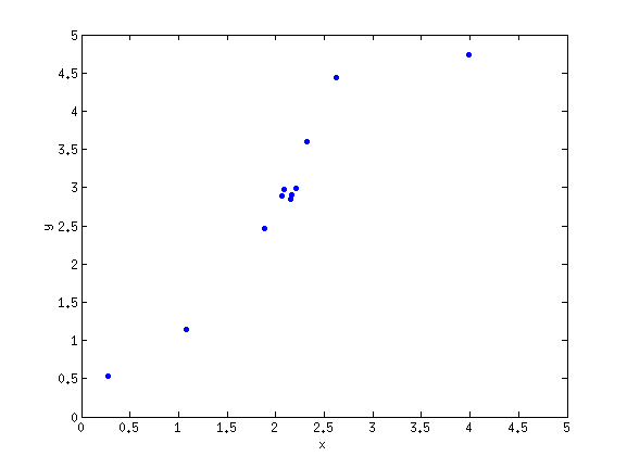

This data looks very linear, aside from the clump from the center, and in fact a standard linear regression would actually work pretty well here. But let’s see what kernel regression does on this data, using a Gaussian kernel with width {$\sigma^2 = 2.5$}: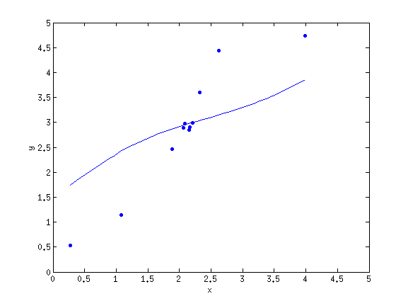

What’s happening is that at each point we predict along the curve, we predict a weighted sum of the other points’ values, where the weighting is determined by the kernel function. However, the points in the center are clustered close enough that we can think of them as having roughly the same location. When we take a weighted sum over all training points, the center point gets added as many times to the sum as there are points clustered in the center; in this case, it has 6 times as much influence over the output as any other point in the training data. The result is that the cluster drags the values of all other points towards its center, and the predictions are highly skewed.

The role of {$\alpha_i$} suggests an immediate remedy to this problem: we could predict much more accurately if the {$\alpha$}’s of those points in the center canceled each other, reducing the influence of the center cluster and treating it more closely to any other point. This is exactly what happens if we run KRR on this dataset: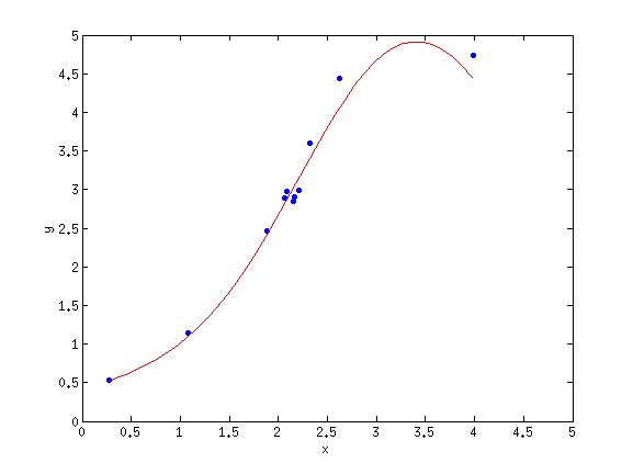

We see that the curve is no longer dominated by the cluster in the center. We can investigate this further by plotting the alphas on the same x-axis as the data:

Although it’s not perfect, we can make two observations about the {$\alpha's$}:

Since {$y$} is increasing as we increase our {$x$} value, {$\alpha_i$} needs to increase as well, to reflect this.
The values of the center points fluctuate between positive and negative; this leads to a canceling out of the “influence” of the cluster values.

1.3 Locally weighted regression

The linear regression weights {$w$} at each point {$x$} in locally weighted regression is given by a regression computed by giving more weight to points near the point, {$x$} , where the prediction is being made and less weight to points further away.

{$\hat{w}(x) = argmin_w \frac{ \sum_i k(x, x_i)(w^Tx_i - y_i)^2 }{\sum_i k(x, x_i)}$}

Of course “nearness” is measured using the kernel function {$k(x,x_i)$} and the summation runs over all {$n$} observations in the training set.

1.4 SVMs: the Smarter Nearest Neighbor ™

This discussion leads naturally to support vector machines (SVM)s. All the kernel methods we’ve discussed so far require storing all of the training examples to use during prediction. If we have a lot of training data, that is a huge burden! As we will see in class, SVMs find a push the “intelligent nearest neighbors” concept even further, by finding a compact set of examples that we can use for prediction: in other words, the most of the {$\alpha_i$} that SVM finds will be zero. The useful examples are called support vectors for reasons that will become clear.

However, SVMs bring a new principle to our discussion, know as max-margin learning. (We first mentioned margins in our discussion of Boosting.) The objective in SVMs is a new type of loss that is not differentiable called the “hinge loss”, and we express the principle of maximizing the margins on training data through constraints on this new objective. The practical result is that the numerical and analytical methods we’ve been using so far for MLE and MAP, (taking the derivative and setting to zero or using gradient descent) will no longer suffice for our needs.

In order to solve the SVM problem, we need concepts from the theory of constrained optimization: namely, Lagrange Duality.

2. Convex Optimization: A Primer

Motivation

In much of class we’ve primarily discussed machine learning through the eyes of statistics: formulating probabilistic models and then optimizing parameters to do MLE or MAP estimation. We’ve also discussed some methods that don’t have a probabilistic interpretation. But regardless, we should have figured out by now that optimization is really, really important for machine learning. For the discriminative methods we’ve discussed so far (linear, logistic regression; boosting, etc.), we can summarize our process as follows:

Formulate a parametric prediction rule, {$h_\theta(\mathbf{x})$}, to predict outputs {$y$} from input {$\mathbf{x}$} using a set of parameters {$\theta$}.
Find the “best” parameters {$\theta$} by minimizing a loss function over the training data, discounted by a penalty regularization term:

{$\theta^\star = \arg\min_\theta \sum_{i=1}^n \mathcal{L}( y_i, h(\mathbf{x}_i)) + R(\theta).$}

The idea is that the loss function measures how well we fit the data, and the penalty function measures how “unrealistic” our current solution is. For example, some of the losses we’ve consider so far are:

Square loss: {$\mathcal{L}(y, \hat{y}) = (y - \hat{y})^2$}, used in linear regression, for {$y \in \mathcal{R}$}
Log loss: {$\mathcal{L}(y,\hat{y}) = log\left(1 + \exp(-y\hat{y})\right),$} used in logistic regression, for {$y \in \{-1,+1\}$}
Exponential loss: {$\exp(-y\hat{y})$}, used in Boosting, for {$y \in \{-1,+1\}$}
0–1 loss: {$\mathcal{L}(y,\hat{y}) = \mathbf{1}[y \ne \hat{y}]$}, used to compute error rate

While a key regularizer we have talked about so far is the result of a gaussian prior: {$R(\mathbf{w}) = \sum_i w_i^2 = ||\mathbf{w}||_2^2,$} which is also known as a Ridge penalty.

With the exception of the {$0-1$} loss, all of these losses are convex functions. Convexity is important for optimization, since convexity implies a single, global minimum: convexity is the only reason why gradient descent is useful. In fact, one of the purposes of the log and exponential losses is to provide a convex upper bound on the {$0-1$} loss. Because {$0-1$} isn’t convex, it is hard to minimize, so we minimize a placeholder instead.

Optimization methods are the key to finding solutions that minimize a given loss, and so far we haven’t run into any problems. In many cases, however what makes it complicated is that sometimes just picking a good model and a good loss function and a good regularizer doesn’t cut it: we need to enforce constraints on the solution that we find. For example,

We might want to find a weight vector {$\mathbf{w}$} that has only positive entries. This would be the constraint {$w_i \ge 0$}, or {$\mathbf{w} \succeq 0$}.
We might be optimizing a matrix {$\mathbf{A}$} to use in a distance based kernel:, {$k(\mathbf{x}, \mathbf{x}') = \exp \{ -(\mathbf{x} - \mathbf{x}')^\top\mathbf{A}(\mathbf{x} - \mathbf{x}')/\sigma^2 \}.$} As discussed in class, in order for the kernel to be valid, we need {$\mathbf{A}$} to be positive semi-definite. This would be the constraint {$\mathbf{A} \succeq 0$}.
We want to use support vector machines, which enforce margin constraints, which will be described in class.

2.1 Optimality conditions

In general, there are many ways to try to solve constrained optimization problems; one of the sneakiest (and easiest) is to rewrite the problem in a clever way so that the constraint disappears. However, at the very least we need some sense of how to test if we’ve found an optimal point for a given problem. These tests are known as optimality conditions.

With an unconstrained convex optimization problem, the optimality conditions are easy. There is only one possible minima to the function, so the minimum is exactly at the point where the derivative is zero. In other words, for convex {$f$}, {$f'(x) = 0 \;\;\rightarrow\;\; x = \min_x f(x).$}

Now suppose we are given the problem, {$\min_x f(x) \quad \textrm{subject to}\quad ax \le b.$} Suppose that {$x^\star = \min_x f(x)$} is the unconstrained solution. Clearly, {$f'(x^\star) = 0$}. But does this mean that {$x^\star$} also minimizes the constrained problem? In other words, do we have any guarantee that {$ax^\star \le b$}? We don’t. Instead, we can guess that at some point the objective of minimizing {$f(x)$} might “be overruled” by the problem of violating the constraint. In order to formulate this intuition precisely, we use a concept called the Lagrangian.

2.2 The Lagrangian

We construct the Lagrangian of a given constrained optimization problem by bringing each constraint into the objective multiplied by a new variable called a Lagrange multiplier. The idea is that the Lagrange multipliers let us explicitly describe that trade-off between minimizing the objective function and satisfying constraints.

Suppose we have the problem:

{$ \begin{array}{ccc} \textrm{minimize} & f_0(x),& \\ \textrm{subject to} & f_i(x) \le 0, & i = 1, \dots, m \\ & h_i(x) = 0, & i = 1, \dots, p \\ \end{array} $}

This is a standard, general formulation of an optimization problem with {$m$} inequality constraints and {$p$} equality constraints. (This is following notation in Boyd & Vanderburg.) The feasible set is the set of all inputs {$x$} that satisfy all of the constraints: our optimization problem is restricted to this feasible set, if it exists. To form the Lagrangian, each one of these constraints gets its own Lagrange multiplier (Technically the multipliers {$\nu_i$} on the equality constraints are Lagrange multipliers and the multipliers {$\lambda_i$} on the inequality constraints are KKT multipliers, but we’ll be a little sloppy and call them all Lagrange multipliers.) We introduce {$m$} variables {$\lambda_i$} for the inequalities, and {$p$} variables {$\nu_i$} for the equalities:

{$ L(x, \lambda, \nu) = f_0(x) + \sum_{i=1}^m \lambda_i f_i(x) + \sum_{i=1}^p \nu_i h_i(x). $}

Why is this useful? Suppose we are optimizing {$f(x)$} subject to the constraint {$ax - b < 0$}, as in our example above. The Lagrangian is, {$L(x,\lambda) = f(x) + \lambda(ax-b).$} Suppose we choose a particular {$\lambda_0$}, where {$\lambda_0 \ge 0$}, so we treat {$\lambda_0$} as constant. Suppose know that a particular {$x = x_0$} is feasible, so it satisfies the constraints of the problem. Then we know that {$ax_0 < b$}, or equivalently {$ax_0 - b \le 0$}. Since {$\lambda_0 \ge 0$}, that means that we have:

{$ \begin{array}{rcl} L(x_0, \lambda_0) & = & f(x_0) + \lambda_0(ax_0-b) = f(x_0) + (\ge 0)(\le 0) \\ & \le & f(x_0) \end{array} $}

In other words, if we have a feasible point {$x_0$} and a given {$\lambda \ge 0$}, then {$L(x_0, \lambda)$} provides a lower bound of the function we’re trying to minimize. This suggests an alternative means of solving our original problem: rather than minimizing {$f(x)$}, we could try to maximize the lower bound. Consider the following function:

{$ \begin{array}{rcl} g(\lambda) & = & \min_x \left( f(x) + \lambda(ax-b) \right), \quad \lambda \ge 0 \\ & \le & f(x_0) + \lambda(ax_0-b) \\ & \le & f(x_0) \end{array} $}

Note that this holds for any feasible point {$x_0$}, which means it must also hold for the solution to the original problem. Therefore, {$g(\lambda) \le f(x^\star), \qquad ax^\star < b, \quad \lambda \ge 0,$} or, in English, the value of {$g(\lambda)$} is a lower bound on the optimal value of the original constrained optimization problem. Thus, {$g(\lambda) = f(x) \;\;\rightarrow\;\; x = x^\star.$} In other words, because {$g(\lambda)$} lower bounds {$f(x)$}, if we find {$g(\lambda)$} that is equal to {$f(x)$} for some {$x$}, we have found the minimum of our function! We are getting dangerously close to something that sounds like an optimality condition.

2.3 Lagrangian Duality

In fact, the function we just defined is called the Lagrange Dual of the optimization problem. For a minimization of the form:

{$ \begin{array}{ccc} \textrm{minimize} & f_0(x),& \\ \textrm{subject to} & f_i(x) \le 0, & i = 1, \dots, m \\ & h_i(x) = 0, & i = 1, \dots, p \end{array} $}

we define the Lagrange dual function as the minimum of the Lagrangian over x: {$g(\lambda, \nu) = \inf_x \left( f_0(x) + \sum_{i=1}^m \lambda_i f_i(x) + \sum_{i=1}^p \nu_i h_i(x) \right),$} where {$\lambda$} and {$\nu$} are known as the dual variables. (Note that just as we said {$x$} was feasible if it met the constraints of the primal problem, we say {$(\lambda,\nu)$} is dual feasible if {$\lambda_i \ge 0$}.) Now, for a given {$\lambda \succeq 0$}, then we have that {$g(\lambda, \nu) \le f(x^\star).$} Thus, we define the Lagrange dual problem as:

{$ \begin{array}{ccc} \textrm{maximize} & g(\lambda, \nu),& \\ \textrm{subject to} & \lambda_i \ge 0, & i = 1, \dots, m \end{array} $}

This is the problem of maximizing the lower bound determined by the dual function. The neat part of this is that if {$f$} is convex and certain conditions hold for the constraints, then the maximum of the dual problem is exactly the minimum of the primal function. This is known as strong duality.

2.4 KKT Conditions + Complementary Slackness

Why was all of this mathematical mishmosh necessary? Until now, we had no way of determining whether or not we had found an optimal point for our function. However, armed with the Lagrange dual function, we can see that, {$g(\lambda^\star, \nu^\star) = f_0(x^\star) \;\;\rightarrow\;\; (x^\star, \lambda^\star, \nu^\star) \textrm{ constitute an optimal solution}.$} But specifically, what does the equality in the above equation imply? There are several important consequences. First, we note that for the two values to be equal,

{$ \begin{array}{rcl} g(\lambda^\star, \nu^\star) & = & \inf_x L(x, \lambda^\star, \nu^\star) \\ & = & f_0(x^\star) + \sum_{i=1}^m \lambda_i^\star f_i(x^\star) + \sum_{i=1}^p \nu_i h_i(x^\star) \\ & = & f_0(x^\star). \end{array} $}

which means that {$ \sum_{i=1}^m \lambda_i^\star f_i(x^\star) + \sum_{i=1}^p \nu_i h_i(x^\star) = 0.$} However, by definition of feasibility, {$h_i(x^\star) = 0$}. Since each term in the sum over {$\lambda_i^\star$} is less than zero, we are left with the fact that: {$\forall i: \quad \lambda_i^\star f_i(x^\star) = 0.$} In other words, {$ \lambda_i^\star > 0 \;\;\rightarrow\;\; f_i(x^\star) = 0, \qquad f_i(x^\star) < 0 \;\;\rightarrow\;\; \lambda_i^\star = 0,$} which says that the {$i$}’th optimal Lagrange multiplier is zero unless the {$i$}’th constraint is active (meaning that this constraint is tight) at the optimum. This relationship is called complementary slackness, and it is this condition that is critical to the “support vector” concept in SVMs!

Another conclusion we can make is that since {$x^\star$} minimizes {$L(x,\lambda,\nu)$} over {$x$}, the gradient of {$L$} with respect to {$x$} must be zero, i.e. {$\nabla f_0(x^\star) + \sum_{i=1}^m \lambda_i^\star \nabla f_i(x^\star) + \sum_{i=1}^p \nu_i^\star \nabla h_i(x^\star) = 0.$}

Together with complementary slackness and the requirements for primal and dual feasibility, these form the Karush-Kuhn-Tucker (KKT) conditions, which completely specify optimality conditions for constrained optimization problems with strong duality. Hooray!

2.5 Example in one dimension

Let’s make this concrete with a very specific example.

Suppose we have the objective function {$f_0(x) = \frac{1}{2}cx^2$}, and the constraint {$f_1(x) = ax - b$}. The primal form of this problem is:

{$ \textrm{minimize} \quad \frac{1}{2}cx^2 \quad \textrm{subject to} \quad ax - b \le 0 $}

Note that in order for this to be convex, we must have {$c \ge 0$}. To solve this, we’re going to use Lagrange duality. We form the Lagrangian by adding a single Lagrange multiplier for the single constraint:

{$L(x,\lambda) = \frac{1}{2}cx^2 + \lambda(ax - b).$}

Now, let’s write down the Lagrange dual function by minimizing {$L$} with respect to {$x$}:

{$g(\lambda) = \min_x L(x,\lambda) = \min_x \frac{1}{2}cx^2 + \lambda ax - \lambda b$}

To minimize this function which is unconstrained with regards to {$x$}, we take the derivative and set to zero:

{$ cx + \lambda a = 0 \;\;\rightarrow\;\; x = -\lambda \frac{a}{c}. $}

To get the formula for {$g(\lambda)$}, we plug back in this minimizing value for {$x$}:

{$ \begin{array}{rcl} g(\lambda) & = & \frac{1}{2}c\left(-\lambda \frac{a}{c}\right)^2 + \lambda a \left(-\lambda \frac{a}{c}\right) - \lambda b\\ & = & \frac{-a^2}{2c}\lambda^2 - \lambda b. \end{array} $}

So this gives us the Lagrange dual problem:

{$ \begin{array}{ccc} \textrm{maximize} & \frac{-a^2}{2c}\lambda^2 - \lambda b& \\ \textrm{subject to} & \lambda \ge 0. \end{array} $}

How do we solve this? Well, let’s try maximizing without constraints and then seeing if the unconstrained maximum is also dual feasible. So, we take the derivative and set to zero:

{$ \frac{-a^2}{c}\lambda - b = 0 \;\;\rightarrow\;\; \lambda^\star = \frac{-bc}{a^2}. $}

Note that if {$b < 0$}, then {$\lambda^\star \ge 0$} and thus is a dual feasible solution to the problem. So, what we see is that if {$b < 0$}, then solving the problem is very easy: we can find the solution to the dual problem using a simple “guess and check” technique! Now, since {$g(\lambda^\star) = f(x^\star)$}, we can plug back in our formula for {$x$} and get the corresponding primal value:

{$x^\star = -\lambda^\star \frac{a}{c} = \frac{bca}{a^2c} = \frac{b}{a},$}

which, as it happens, is exactly the x-intercept of the equation {$ax = b$}.

Intuitively, this solution makes sense: the feasible region defined by the constrain {$ax - b \le 0$} is the region on the x axis where the line {$ax = b$} takes on values below zero.

We can plot this for the values {$a=2$}, {$b=-5$}, and {$c=1$} below: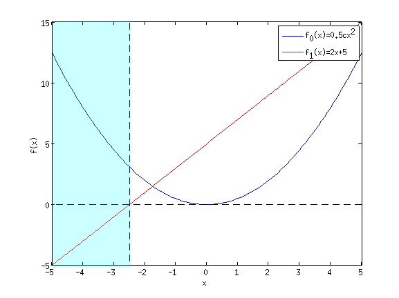

In this example, the blue line is our minimization objective, and the red line is the constraining line {$ax - b = 0$}. This line passes through the x-axis at {$x=-2.5$}. Thus, the feasible region is shaded in blue. Minimizing {$f_0(x)$} in the shaded region is therefore simply taking the rightmost point, which is the x-intercept at {$x=-2.5$}.

SVM Prep