On this page… (hide)

1. The Big Picture
2. Example Problems
1. 2.1 Simple numerical example
2. 2.2 Multivariate Gaussian Estimation
3. 2.3 Poisson distribution
4. 2.4 Bias-Variance Decomposition in Regression

1. The Big Picture

Here we’re going to look at examples of point estimation on 3 different models. In general, when we say “model” we mean some set of parameters, and we want to find good values of these parameters, by maximizing the likelihood of the data (MLE) and potentially including prior knowledge we could have about the parameters (MAP).

Simple custom distribution {$P(X \mid \theta)$}
Objective: Use MLE/MAP formulas to find a “good” {$\theta$}
Multivariate Gaussian distribution {$P(X \mid \mu, \Sigma)$}
Objective: MLE estimation of {$\mu$} and {$\Sigma$}, then MAP of {$\mu$} with a Gaussian prior
Poisson distribution {$P(X\mid \lambda)$}
Objection: MLE estimation of {$\lambda$}, then MAP estimation with a Gamma prior
Bias-Variance Decomposition in Regression
Model: {$y = f(x) = w_0$}, with single parameter {$w_0$}
Objective: Least squares formula stipulates what constitutes “good” {$w_0$}

2. Example Problems

2.1 Simple numerical example

The graphs below show likelihood and prior of a model parameter {$\theta$}, which is discretized into 5 values.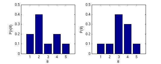

Left: Likelihood. Right: Prior.

What is the MLE of {$\theta$}?

{$ \hat{\theta}_{MLE} = \arg\max_\theta P(X \mid \theta) = 2 $}

What is the MAP estimate of {$\theta$}?

{$ \hat{\theta}_{MAP} = \arg\max_\theta P(X \mid \theta)P(\theta) = 4 $}

What is the value of the posterior at {$\hat{\theta}_{MAP}$}?

{$ P(\hat{\theta}_{MAP} \mid X) = \frac{P(X \mid \hat{\theta}_{MAP})P(\hat{\theta}_{MAP})}{P(X)} = \frac{P(X \mid \hat{\theta}_{MAP})P(\hat{\theta}_{MAP})}{\sum_\theta P(X \mid \theta)P(\theta)} = \frac{0.2*0.3}{0.17} = 0.3529 $}

What is the posterior mean of {$\theta$}?

{$ \mathbb{E}_{P(\theta \mid X)}[\theta] = \sum_\theta \theta P(\theta \mid X) = \frac{1}{0.17} \sum_\theta \theta P(X \mid \theta)P(\theta) = \frac{0.51}{0.17} = 3 $}

2.2 Multivariate Gaussian Estimation

The formula for the multivariate Gaussian is much like that of the univariate Gaussian. Consider the p-variate case where {$X = (X_1, X_2, \ldots, X_p)$}:

{$ P(X \mid \mu, \Sigma) = \frac{1}{(2\pi)^{p/2} |\Sigma|^{1/2}} \exp \Bigg(-\frac{1}{2} (X - \mu)^T \Sigma^{-1}(X - \mu) \Bigg). $}

{$\Sigma$} is called the covariance matrix. Expanding all the vectors and matrices in this formula to clarify what each contains:

{$ P\left( \left.\left[ \begin{array}{c} X_1 \\ \vdots \\ X_p \end{array} \right]\;\; \right\vert \;\; \left[ \begin{array}{c} \mu_1 \\ \vdots \\ \mu_p \end{array} \right], \left[ \begin{array}{ccc} \sigma_{11} & \ldots & \sigma_{1p} \\ \vdots & \vdots & \vdots \\ \sigma_{p1} & \ldots & \sigma_{pp} \end{array} \right] \right) = (2\pi)^{-p/2} \left| \begin{array}{ccc} \sigma_{11} & \ldots & \sigma_{1p} \\ \vdots & \vdots & \vdots \\ \sigma_{p1} & \ldots & \sigma_{pp} \end{array} \right|^{−1/2} e^{\Omega} $}

where

{$\Omega = \Bigg(-\frac{1}{2} \left[ \begin{array}{ccc} (X_1 - \mu_1) & \ldots & (X_p - \mu_p) \end{array} \right] \left[ \begin{array}{ccc} \sigma_{11} & \ldots & \sigma_{1p} \\ \vdots & \vdots & \vdots \\ \sigma_{p1} & \ldots & \sigma_{pp} \end{array} \right]^{-1} \left[ \begin{array}{c} X_1 - \mu_1 \\ \vdots \\ X_p - \mu_p \end{array} \right] \Bigg)$}

where {$\sigma_{ij} = cov(X_i, X_j) = \mathbb{E}_X[(X_i - \mu_i)(X_j - \mu_j)]$}, hence {$\sigma_{ii} = var(X_i) = \mathbb{E}_X[(X_i - \mu_i)^2]$}. In the exercises below, we’ll consider how to best set the parameters of a bivariate Gaussian, {$P(X_1, X_2 \mid \mu_1, \mu_2, \sigma_{11}, \sigma_{22}, \sigma_{12})$}, on the basis of a dataset {$D = \left\{(x_{1}^{(1)}, x_{2}^{(1)}), \ldots, (x_{1}^{(n)}, x_{2}^{(n)})\right\} $} which contains {$n$} data points.

Compute the MLE of {$\mu_1$}, {$\sigma_{11}$}, and {$\sigma_{12}$} for the bivariate Gaussian. (Your answer should be in terms of the data in {$D$}).

(:answiki:) We will show the result for the multivariate case and interpret it in the 2D case. Just like in the 1D case, the procedure is the following:

Form the likelihood of the data, {$\prod_{i = 1}^m P_i$}, where each {$P_i$} is in the form of a bivariate Gaussian
Take the log of the likelihood to make the math easier later
Take the derivative of the log likelihood with respect to the parameter of interest, then set that equal to 0, and finally solve for the parameter of interest.

Here the parameters we want to estimate are a vector ({$\mu$}) and a matrix ({$\Sigma$}). We could develop the likelihood to expose {$\mu_1,\mu_2,\sigma_{11},\sigma_{22},\sigma_{12}$} and take derivatives w.r.t. each of them, but let’s use a faster method: we are going to take derivatives with respect to the vector {$\mu$} and the matrix {$\Sigma$}:

When {$f(\mu)$} is a scalar, {$\frac{df(\mu)}{d\mu}$} is a vector (each component is {$\frac{df}{d\mu_i}$})
When {$f(\mu)$} is a vector {$(f_1(\mu),\ldots,f_K(\mu))$} (where each {$f_i$} is scalar), {$\frac{df(\mu)}{d\mu}$} is a matrix: each row {$i$} is the vector {$\frac{df_i}{d\mu}$} as defined above.
When {$f(\Sigma)$} is a scalar, {$\frac{df(\mu)}{d\Sigma}$} is a matrix (where each component {$(i,j)$} is {$\frac{df(\mu)}{d\Sigma_{i,j}}$})

Here are useful derivation formulas that we will use. Make sure you understand the dimensions using the 3 facts above. When {$x$} is a vector and {$A$} and {$B$} squared matrices, we have:

{$\frac{d(Ax)}{dx}=A$} (analog to {$\frac{d(ax)}{dx}=a$} in 1D)
{$\frac{d(x^TAx)}{dx}=2x^TA$} (analog to {$\frac{d(ax^2)}{dx}=2ax$} in 1D)
{$\frac{d(Tr(AB))}{dB}=A^T$}
{$\frac{d(\log |A|)}{dA} = A^{-1}$}

MLE of the mean (:centereq:) {$\begin{array}{rl} \log P(D \mid \mu,\Sigma) &= -\frac{Nd}{2} \log(2\pi) - \frac{N}{2} \log |\Sigma| - \frac{1}{2} \sum_{i=1}^N (x_i-\mu)^T \Sigma^{-1}(x_i-\mu) \\ \frac{d\log P(D \mid \mu,\Sigma)}{d\mu} &= \sum_{i=1}^N (x_i-\mu)^T \Sigma^{-1} \end{array}$} (:centereqend:) By setting this derivative to zero (which means we are setting all its components to 0, since it is a vector), we have the following: (:centereq:) {$\mu_{MLE} = \frac{1}{N} \sum_{i=1}^N x_i$} (:centereqend:)

MLE of the variance
The most dreadful term is the sum containing {$\Sigma^{-1}$}. We can rewrite it as follows: (:centereq:){$\begin{array}{rl}\sum_i (x_i-\mu)^T \Sigma^{-1} (x_i - \mu) =& \sum_i Tr((x_i-\mu)^T \Sigma^{-1} (x_i - \mu)) \\ =& \sum_i Tr(\Sigma^{-1}(x_i - \mu)(x_i-\mu)^T ) \end{array}$}(:centereqend:) We used the fact that the trace is invariant under circular permutation. Now we could almost use the derivation formula number (3). Actually we can if we consider {$P(D\mid \mu,\Sigma)$} as a function of {$\Sigma^{-1}$} instead of {$\Sigma$}: we can indeed write {$-\log|\Sigma| = \log(\frac{1}{|\Sigma|}) = \log|\Sigma^{-1}|$}. The likelihood reaches its maximum when the derivative w.r.t. {$\Sigma^{-1}$} is zero:

(:centereq:){$\frac{d\log P(D \mid \mu,\Sigma)}{d(\Sigma^{-1})} = 0 = \frac{N}{2}\Sigma - \frac{1}{2}\sum_i (x_i-\mu)(x_i-\mu)^T$}(:centereqend:)

(:centereq:) {$\Sigma_{MLE} = \frac{1}{N} \sum_i (x_i- \mu)(x_i - \mu)^T$} (:centereqend:)

This turns out to be the empirical covariance matrix of the data: we will study its properties and meaning later on, when we will introduce PCA. Using the two MLE formulas we just found, we can write the coefficients of {$\mu$} and {$\Sigma$} in 2D as follows:

(:centereq:) {$ \begin{array}{rl} \hat{\mu}_{1_{MLE}} & = \frac{1}{m} \sum_{i = 1}^m x_1^{(i)} \\ \hat{\sigma}_{11_{MLE}} & = \frac{1}{m} \sum_{i = 1}^m (x_1^{(i)} - \hat{\mu}_1)^2 \\ \hat{\sigma}_{12_{MLE}} & = \frac{1}{m} \sum_{i = 1}^m (x_1^{(i)} - \hat{\mu}_1)(x_2^{(i)} - \hat{\mu}_2) \end{array} $} (:centereqend:) (:answikiend:)

Now suppose we add a prior on {$\mu$} that is also a bivariate Gaussian: {$P(\mu_1, \mu_2 \mid \mu_{1_0}, \mu_{2_0}, \sigma_{11_0}, \sigma_{22_0}, \sigma_{12_0})$}.

Compute the MAP estimate of {$\mu = [\mu_1, \mu_2]^T$} using this prior.

The intermediate steps are not shown here, but the general procedure is to form the likelihood*prior, {$\prod_{i = 1}^m P_i*P(\mu)$}, where each {$P_i$} is in the form of a bivariate Gaussian, then take the log of this expression to make the math easier later, then take the derivative with respect to {$\mu_1$}, then set that equal to 0, and finally solve for {$\mu$}.

(:centereq:) {$ \hat{\mu}_{MAP} = (\Sigma_0^{-1} + m\Sigma^{-1})^{-1}\Bigg(\mu_0^T\Sigma_0^{-1} + \sum_{i = 1}^m x^{(i)}\Sigma^{-1}\Bigg) $} (:centereqend:)

where {$\mu_0 = [\mu_{1_0}, \mu_{2_0}]^T$} and {$x^{(i)} = [x_1^{(i)}, x_2^{(i)}]^T$} (the i-th data point).

MLE for the general multivariate case is detailed on Wikipedia, if you’re curious.

2.3 Poisson distribution

The Poisson distribution can be useful to model how frequently an event occurs in a certain interval of time (packet arrival density in a network, failures of a machine in one month, customers arriving at a waiting line…). Like any other distribution, the parameter (here {$\lambda$}) can be estimated from some measurements/experiences. The pmf is the following:

{$P(X \mid \lambda) = \frac{\lambda^X e^{-\lambda}}{X!}$}

Show that maximum-likelihood estimate of {$\lambda$} is {$\hat{\lambda} = \frac{1}{n} \sum_i X_i$}.
Show that the MLE of {$\lambda$} is unbiased: show that {$\mathbb{E}_X[\hat{\lambda}(X)] = \lambda$}
To express the MAP estimate of {$\lambda$} we need to incorporate a prior term. The idea is to use a prior distribution that will facilitate the calculations: here the conjugate prior of the Poisson distribution is the Gamma distribution:
{$\Gamma(\lambda \mid \alpha,\beta) = \frac{\beta^{\alpha}}{\Gamma(a)}\lambda^{\alpha-1}e^{-\beta\lambda}, \;\;\lambda > 0$}
Compute the posterior distribution. Hint: show that it has the same form as the prior (hence the expression “conjugate prior”).
Using the posterior you just computed, find the analytic expression of the MAP estimate. Not only does the posterior have a nice closed-form expression, but it also gives us an idea of how the likelihood updates MLE.

2.4 Bias-Variance Decomposition in Regression

Suppose we decide to fit the simplest regression model {$y = f(x) = w_0$}, which is constant for all {$x$}, to some data. Now, suppose the actual underlying model that generated the data is {$y = g(x) = ax$}, where {$a$} is a constant. In other words, we are modeling the underlying linear relation with a constant model.

For this problem, we will consider all data to be noise-free. Consider a particular training set {$D$} where the inputs are {$ \{x_1, x_2\} $} and the responses are {$y_1 = a x_1, y_2 = a x_2$}, as shown in the figure below where {$g(x)$} and {$f(x)$} are fit using least squares.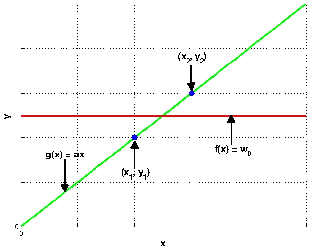

The curves {$\hat{f}_D(x)$} and {$g(x)$}

Assuming standard least squares fitting, for what values of {$a$} will the bias of our model ({$f(x)$}) be 0? For what values of {$a$} will the variance be 0?

Bias and variance are 0 for {$a = 0$}, since in that case the estimated model is the line {$y = 0$}, which is exactly the true model, regardless of the sample positions of {$x_1$} and {$x_2$}.

Compute the least squares estimate of {$f(x)$} given dataset {$D$}: {$\hat{f}_D(x) = \hat{w}_0$}. (Your answer should be in terms of {$x_1$}, {$x_2$}, and {$a$}.)

(:centereq:) {$\hat{w}_0 = \arg\min_{w_0} [(w_0 - ax_1)^2 + (w_0 - ax_2)^2]$} (:centereqend:)

Taking the derivative with respect to {$w_0$}: (:centereq:) {$0 = 2(\hat{w}_0 - ax_1) + 2(\hat{w}_0 - ax_2)$} (:centereqend:) (:centereq:) {$\hat{w}_0 = \frac{a(x_1 + x_2)}{2}$} (:centereqend:)

For a single test point {$x$}, compute the squared error of our estimate for this point given dataset {$D$}: {$err(\hat{f}_D, x) = (\hat{f}_D(x) - g(x))^2$}? (Your answer should be in terms of {$x_1$}, {$x_2$}, {$a$}, and {$x$}.)

(:centereq:) {$(\hat{w}_0 - ax)^2 = \Bigg(\frac{a(x_1 + x_2)}{2} - ax \Bigg)^2$} (:centereqend:)

Assuming {$p(x) \sim \mathcal{U}[0,1]$} (uniform on [0,1]), compute the expected squared error given dataset {$D$}: {$err(\hat{f}_D) = \mathbb{E}_x[err(\hat{f}_D, x)]$}. (Your answer should be in terms of {$x_1$}, {$x_2$}, and {$a$}, and should not contain any integrals.)

(:centereq:) {$ \begin{align*} err(\hat{f}_D) & = \int_x (\hat{w}_0 - ax)^2 p(x) dx \\ & = \int_0^1 (\hat{w}_0 - ax)^2 dx \\ & = \hat{w}_0^2 - \hat{w}_0a + \frac{a^2}{3} \\ & = a^2 \Bigg(\frac{(x_1 + x_2)^2}{4} - \frac{x_1 + x_2}{2} + \frac{1}{3} \Bigg) \end{align*}$} (:centereqend:)

Assuming {$p(x_1) \sim \mathcal{U}[0,1]$} and {$p(x_2) \sim \mathcal{U}[0,1]$}, compute the expected squared error (the average over datasets): {$err(\hat{f}) = \mathbb{E}_D[err(\hat{f}_D)]$}. (Your answer should be in terms of {$a$} only, and should not contain any integrals.)

(:centereq:) {$ \begin{array}{rl} err(\hat{f}) &= \int_0^1 \int_0^1 err(\hat{f}_D) p(x_1) p(x_2) dx_1 dx_2 \\ &= \int_0^1 \int_0^1 err(\hat{f}_D) dx_1 dx_2 \\ &= \int_0^1 \int_0^1 a^2 \Bigg(\frac{(x_1 + x_2)^2}{4} - \frac{x_1 + x_2}{2} + \frac{1}{3} \Bigg) dx_1 dx_2 \end{array} $} (:centereqend:)

Let’s recall the results of three simpler double integrals in order to cleanly solve this large one: (:centereq:) {$ \; $ \begin{align*} \int_0^1 \int_0^1 x_1 dx_1 dx_2 & = \int_0^1 \int_0^1 x_2 dx_1 dx_2 = \frac{1}{2} \\ \int_0^1 \int_0^1 x_1^2 dx_1 dx_2 & = \int_0^1 \int_0^1 x_2^2 dx_1 dx_2 = \frac{1}{3} \\ \int_0^1 \int_0^1 x_1 x_2 dx_1 dx_2 & = \frac{1}{4} \end{align*} $ \; $} (:centereqend:)

Plugging these into our larger double integral: (:centereq:) {$ err(\hat{f}) = a^2 \Bigg(\frac{\frac{1}{3} + 2*\frac{1}{4} + \frac{1}{3}}{4} - \frac{(\frac{1}{2} + \frac{1}{2})}{2} + \frac{1}{3} \Bigg) = \frac{a^2}{8} $} (:centereqend:)

Compute the expected fit: {$\overline{f}(x) = \overline{w}_0 = \mathbb{E}_D[\hat{f}_D]$}.

(:centereq:) {$ \begin{array}{rl} \overline{f}(x) & = \int_0^1 \int_0^1 \hat{w}_0 p(x_1) p(x_2) dx_1 dx_2 \\ & = \int_0^1 \int_0^1 \hat{w}_0 dx_1 dx_2 \\ & = \int_0^1 \int_0^1 \frac{a(x_1 + x_2)}{2} dx_1 dx_2 \\ & = \frac{a(\frac{1}{2} + \frac{1}{2})}{2} \\ & = \frac{a}{2} \end{array} $} (:centereqend:)

Compute the bias-squared: {$bias^2(f) = \mathbb{E}_x[(g(x) - \overline{f}(x))^2]$}. (Your answer should be in terms of {$a$} only, and should not contain any integrals.)

(:centereq:) {$ \begin{array}{rl} bias^2{f} & = \int_0^1 (g(x) - \overline{f}(x))^2 dx \\ & = \int_0^1 \Bigg(ax - \frac{a}{2} \Bigg)^2 dx \\ & = \left.\frac{a^2x^3}{3} - \frac{2a^2x^2}{4} + \frac{a^2x}{4} \right|_0^1 \\ & = \frac{a^2}{12} \end{array} $} (:centereqend:)

Compute the variance: {$var(f) = \mathbb{E}_x[\mathbb{E}_D[(\hat{f}_D(x) - \overline{f}(x))^2]]$}. (Your answer should be in terms of {$a$} only, and should not contain any integrals.)

(:centereq:) {$ \begin{array}{rl} var(f) & = \int_0^1 \int_0^1 \int_0^1 (\hat{f}_D(x) - \overline{f}(x))^2 dx_1 dx_2 dx \\ & = \int_0^1 \int_0^1 \int_0^1 \Bigg(\frac{a(x_1 + x_2)}{2} - \frac{a}{2} \Bigg)^2 dx_1 dx_2 dx \\ & = \int_0^1 \int_0^1 \int_0^1 \frac{a^2}{4} (x_1 + x_2 - 1)^2 dx_1 dx_2 dx \\ & = \int_0^1 \int_0^1 \left.\frac{a^2}{4} \frac{(x_1 + x_2 - 1)^3}{3} \right|_0^1 dx_2 dx \\ & = \int_0^1 \int_0^1 \frac{a^2}{12} (x_2^3 - (x_2 - 1)^3) dx_2 dx \\ & = \int_0^1 \left.\frac{a^2}{12} \Bigg(\frac{x_2^4}{4} - \frac{(x_2 - 1)^4}{4} \Bigg) \right|_0^1 dx \\ & = \int_0^1 \frac{a^2}{12} \Bigg(\frac{1}{4} + \frac{1}{4} \Bigg) dx \\ & = \frac{a^2}{24} \end{array} $} (:centereqend:)